
HOMER
Software for motif discovery and next-gen sequencing analysis
Creating and Normalizing Hi-C interaction Matrices
The most basic way to represent Hi-C data is in matrix
format, where the number of interactions can be reported
between sets of regions. Since it's difficult to
extract this data from the raw mapped reads, HOMER
provides tools create matrices from tag directories.
Most Hi-C tasks in HOMER revolve around the analyzeHiC
command. Below is a description of how to use it to
create matrices. analyzeHiC requires a Hi-C
tag directory (direction on creating one can be found here). Many of the
commands below require a "Hi-C background model" to
efficiently normalize and calculate expected interaction
counts (If one doesn't exist, it will be created
automatically). Creation of Hi-C background models
can be found here.
Quick Note about Hi-C Analysis
Hi-C is an unbiased assay of chromatin conformation, resulting in even read coverage across the entire genome. This, coupled with the fact that most Hi-C reads describe interactions at close linear distance along the chromosomes, results in relatively sparse read coverage for interactions between individual restriction fragments separated by great distance. This makes it difficult to find high-resolution interactions across long distances. To help describe how distal and/or inter-chromosomal regions co-localize, two general approaches are utilized:
- Increase the size of the regions [i.e. decrease the resolution] to boost the number of Hi-C reads used for interaction analysis. This is the most common and simplest technique used by most approaches (including HOMER). It's much easier to identify significant inter-chromosomal interactions between regions that are 100kb in size than regions that are only 5kb in size (essentially 20x more Hi-C reads to work with).
- Compare the profile of interactions regions participate in when comparing regions. The best example of this is calculating the correlation coefficient of the interaction profiles between two regions. The idea is that if two regions share interactions with several other regions, they are probably similar themselves (even if they do not have direct interaction evidence between them). This forms the basis of the PCA analysis, and uses the transitive property to link regions. If A interacts with C and D, and B interactions with C and D, perhaps A and B interact as well.
Running analyzeHiC
Changing the Resolution and Super Resolution
If the output requires normalization, HOMER will construct a background model for the specified resolution. If it is the first time you've used the designated resolution, HOMER will generate a background model (more on that below). For small resolutions, this can take a while...
HOMER uses two (related) notions of resolution. The first, "-res <#>" represents how frequent the genome is divided up into regions. The second, the super resolution "-superRes <#>" (poorly named), represents how large the region is expanded when counting reads. Usually the "-res <#>" should be smaller than the "-superRes <#>". For example a res of 50000 and a superRes of 100000 would mean that HOMER will analyze the regions 0-50k, 50k-100k, 100k-150k etc., but at each region it will look at reads from a region the size of 100k, so it would look at reads from -25k-75k, 25k-125k, 75k-175k, etc. This means HOMER will analyze data with overlapping windows. The principle advantage to this strategy is that you don't penalize features that span boundaries. For example:
analyzeHiC ES-HiC -res 10000 -superRes 20000 > output.10kby20kResolution.txtKeep in mind that the resolution will also dictate the size of the output matrix. The command will warn you if your parameters seem unreasonable...
Specifying specific Regions to Analyze
-start <#> : starting position for analysis
-end <#> : end position for analysis
-pos <chr:start-end> : UCSC browser formatted position - if you're lazy like me, takes place of the -chr/-start/-end
If you only "-chr chr1" and do not specify a start and end, HOMER will simply visualize all of chr1. Regions will be created starting at position 0 to 1*resolution, then from 1*resolution to 2*resolution, etc. (i.e. 0-10kb, 10kb-20kb, 20kb-30kb) If an alternative start is specified, then regions will be created at start+0*resolution to start+1*resolution, start+1*resolution to start+2*resolution, etc (i.e. 205kb-215kb,215kb-225kb,...).
HOMER will normally make a symmetric matrix by default. If you want to specifically look at a matrix between two different regions:
-start2 <#> : starting position for analysis
-end2 <#> : end position for analysis
-pos2 <chr:start-end> : UCSC browser formatted position - if you're lazy like me, takes place of the -chr2/-start2/-end2
-vsGenome : compare to the rest of the genome
NOTE: Don't use -chr2/-start2/-end2/-pos2/-vsGenome unless you specified something with -chr/-start/-end/-pos etc. first.
Using these regions, HOMER will divide them into #-bp regions, where # is the resolution. HOMER doesn't allow you to cherry-pick several regions from different chromosomes. At least not using the -chr, -start, -end, and -pos options. (You could do this with peaks and the -p option).
You can arbitrarily define the regions you want to examine by providing a peak/BED file of the regions. However, these options work a little differently. In the case above (with -chr/-start/-end/-pos), HOMER will chop up the region into resolution sized chunks and perform the analysis. I.e. you provide a locus you want a detailed picture of. When providing a peak file, HOMER will only consider the center of the peak file and the surrounding "resolution-sized" region. It will not chop-up your peaks into resolution-sized chunks (unless you specify the "-chopify" option). In general, the "-p" option is more useful for looking at all CTCF peaks, for example, to see which are interacting. You can provide a peak/BED that effectively tiles a region, in which case it would mimic how -chr/-start/-end/-pos works, but give you the flexibility to define any region(s) you wanted. To specify a peak file containing regions to analyze with analyzeHiC:
-p2 <peak/BED file> : A second peak/BED file for non-symetrical matricies.
Keep in mind that an interaction matrix is probably only useful at 2000 x 2000 points - much bigger you can't really visualize it easily anymore (The file will also get really big...)
Matching the resolution of Peak/BED Files and
Resolution of analyzeHiC
The resulting file will contain only peaks at least 50000 bp from one another. Use this resulting file with analyzeHiC.
Creating an Interaction Matrix
Output Information Options (choose only one ):
-simpleNorm
-norm (default)
-logp
-expected
-rawAndExpected <expectedMatrix filename>
-corr (can be used with any of the above options)
Visualizing the Interaction Matrix
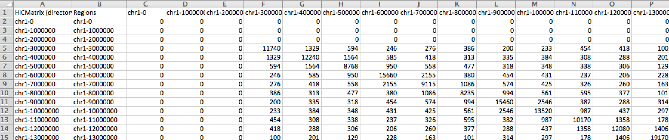
To view the output as a heatmap, open it in Java Tree View (or any other software that generates Heat Maps). You may have to adjust the pixel settings to get the desired level of brightness. If viewing normalized data of observed vs. expected log2 ratios, you may want to view the matrix so that interacting regions are positive (one color) and non-interacting regions are negative (a different color).
By default, analyzeHiC sorts the chromosomes numerically and places the X, Y, and M at the end of the list (You can tell in the example below that the cells are from a male because the X chromosome is lighter than the others...)
Example 1: Raw interactions across the genome at 1 Mb resolution
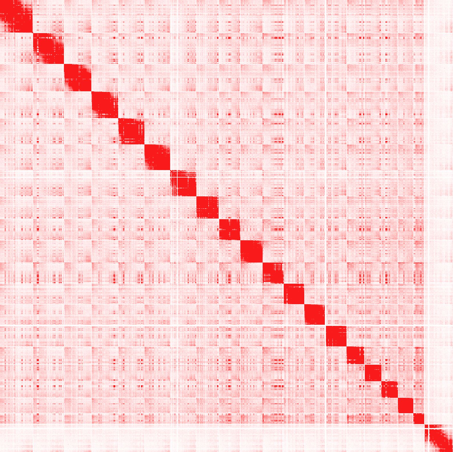
As you can see, interactions are much more frequent within chromosomes than between.
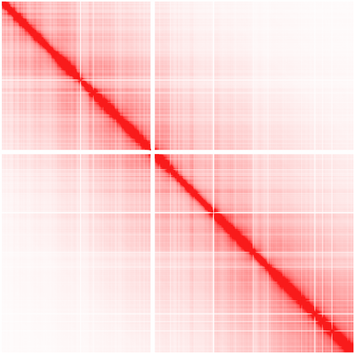
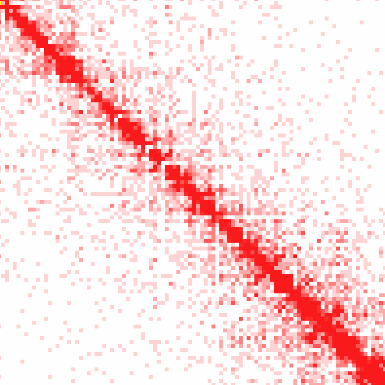
Example 2: Raw interactions across chr1 at 100 kb resolution
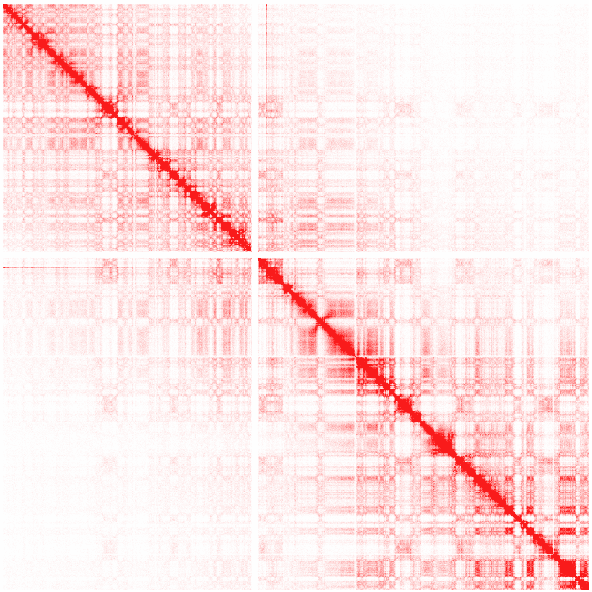
Here you'll start to notice the compartment patterns.
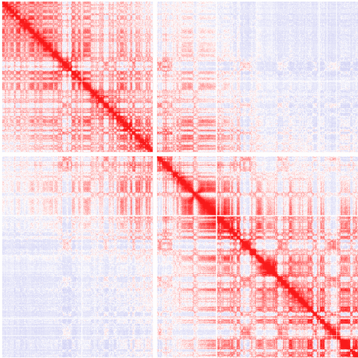
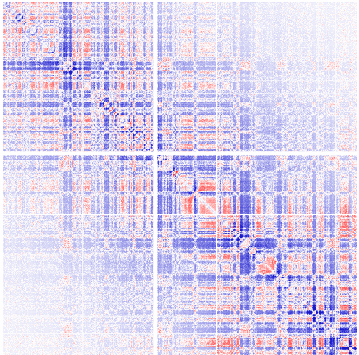
Example 3: Ratio of observed vs. expected interactions across chr1 at 100 kb resolution using simple normalization (normalizing for sequencing coverage only). Visualized as log2 ratios of observed interactions relative to expected interactions (red being positive, blue negative)
Example 4: Ratio of observed vs. expected interactions across chr1 at 1 kb resolution (normalizing for sequencing coverage and distance between loci - this is the default). Visualized as log2 ratios of observed interactions relative to expected interactions (red being positive, blue negative). NOTE: If a 100kb background model does not exist, it will be created the first time (may take some time).
Example 5: You might be curious what the "expected" interactions are from the background model. Use the "-expected" option for that:
analyzeHiC ES-HiC -chr chr1 -res 100000 -expected > outputFile.txt
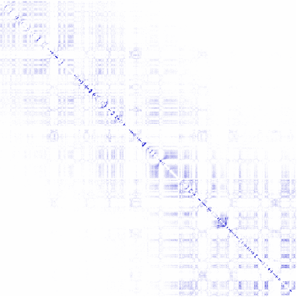
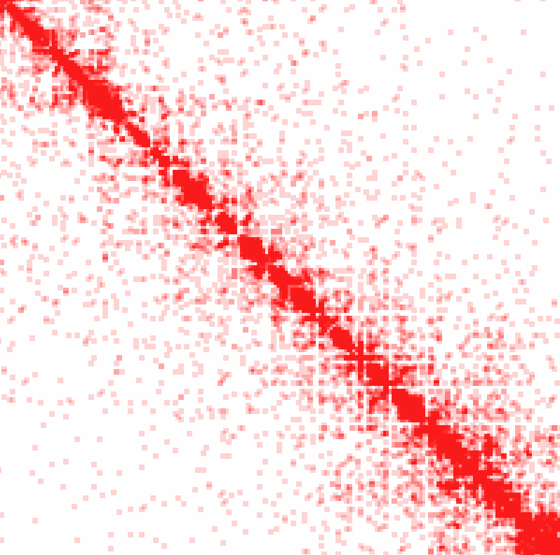
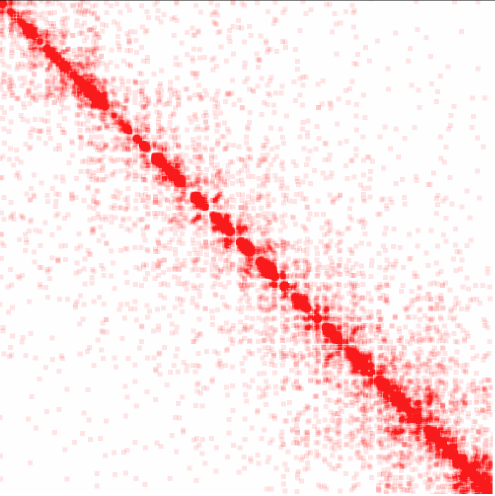
Example 6: log p-values for interactions across chr1 at 100 kb resolution (normalizing for sequencing coverage and distance between loci). More information about the p-value calculation is available in the "Identifying Significant Interactions" section.
As you might notice, most of the significant interactions appear closer to the diagonal where the read coverage is high enough to confidently identify overrepresented interactions.
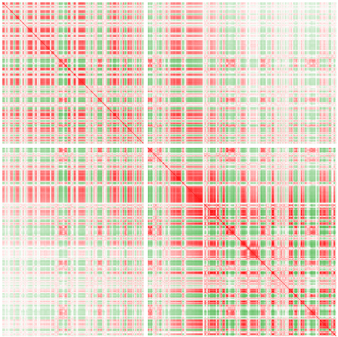
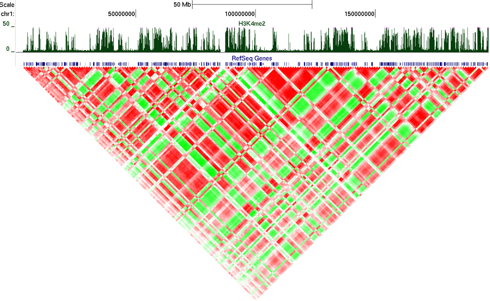
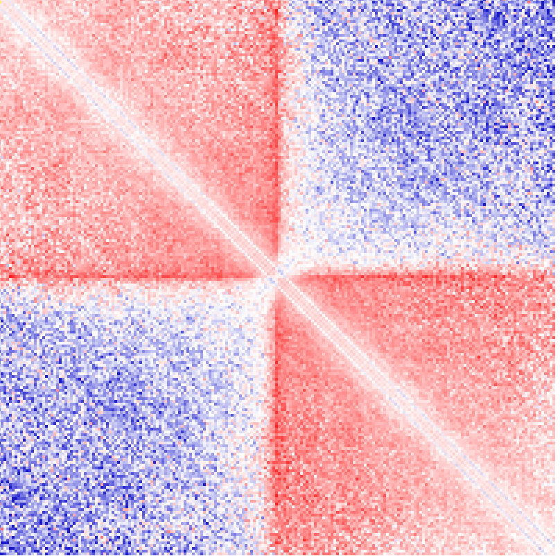
Example 7: Correlation of normalized interaction ratios across chr1 at 100 kb resolution. More about correlation can be found in the "Sub-nuclear compartment analysis/PCA" section. Positive correlation is shown as red, negative correlation as green.
Example 8: Poor man's data integration.
Example 9: Analyzing Peak Files
When analyzing peak files, use the "-p <peak/BED file>". The key difference here is that the matrix that is returned will show each row/column as a peak, and not a continuous section of the genome. Peak regions will be sorted based on their position in the output. For example:
mergePeaks CTCFchr10.peaks.txt -d 50000 > inputPeaks.txt
analyzeHiC ES-HiC -p inputPeaks.txt -res 50000 > outputFile.txt
Using -res and -superRes
The "-superRes <#>" option is basically a way to make moving windows (explained in more detail at the beginning of this section). In summary, instead of analyzing the data at resolution of 10kb for every 10kb of sequence, you can analyze at a resolution of 10kb (-superRes) but perform that analysis every 1kb of sequence (-res) Normally, you want to superRes to be larger than the resolution, or the same (default). The idea is that it will smooth out features and be more resilient to boundary effects. Below is an example of how it looks with raw interactions.
analyzeHiC ES-HiC -res 10000 -superRes 10000 -pos chr1:20000000-21000000 -raw > output.txt
analyzeHiC ES-HiC -res 5000 -superRes 10000 -pos chr1:20000000-21000000 -raw > output.txt
analyzeHiC ES-HiC -res 1000 -superRes 10000 -pos chr1:20000000-21000000 -raw > output.txt
Creating 2D Histograms of Interactions
To make a 2D histogram, you MUST specify a peak file ("-p <peak/BED file>"), a total size of the interaction matrix ("-size <#>"), and the histogram resolution ("-hist <#>") ("-hist" takes the place of "-res" in this case).
i.e. analyzeHiC ES-HiC -size 1000000 -hist 10000 -p tssPositions.txt > output2dHistogram.txt
If -logp, -simpleNorm, etc. are used then those values will be added together for use in the histogram. If you choose to view too many peaks, too large of a size or small of a resolution, the memory requirements can get large, so be careful.
For example:
analyzeHiC ES-HiC -size 1000000 -hist 5000 -p CTCFpeaks.chr10.bed > output.txtIn this example you can see how CTCF tends to sit at the boundaries between interconnected "domains".
Visualizing with TreeView:
Command Line Options for analyzeHiC
Usage: analyzeHiC <PE tag directory> [options]...
Resolution Options:
-res <#> (Resolution of matrix in bp or use "-res site" [see below], default: 10000000)
-superRes <#> (size of region to count tags, i.e. make twice the res, default: same as res)
Region Options:
-chr <name> (create matrix on this chromosome, default: whole genome)
-start <#> (start matrix at this position, default:0)
-end <#> (end matrix at this position, default: no limit)
-pos chrN:xxxxxx-yyyyyy (UCSC formatted position instead of -chr/-start/-end)
-chr2 <name>, -start2 <#>, -end2 <#>, or -pos2 (Use these positions on the
y-axis of the matrix. Otherwise the matrix will be sysmetric)
-p <peak file> (specify regions to make matrix, unbalanced, use -p2 <peak file>)
-vsGenome (normally makes a square matrix, this will force 2nd set of peaks to be the genome)
-chopify (divide up peaks into regions the size of the resolution, default: use peak midpoints)
-fixed (do not scale the size of the peaks to that of the resolution)
-pout <filename> (output peaks used for analysis as a peak file)
Interaction Matrix Options:
-norm (normalize by dividing each position by expected counts [log ratio], default)
-zscoreNorm (normalize log ratio by distance dependent stddev, add "-nolog" to return linear values)
-logp (output log p-values)
-simpleNorm (Only normalize based on total interactions per location [log ratio], not distance)
-raw (report raw interaction counts)
-expected (report expected interaction counts based on average profile)
-corr (report Pearson's correlation coeff, use "-corrIters <#>" to recursively calculate)
-corrDepth <#> (merge regions in correlation so that minimum # expected tags per data point)
-o <filename> (Output file name, default: sent to stdout)
-cluster (cluster regions, uses "-o" to name cdt/gtr files, default: out.cdt)
-clusterFixed (clusters adjacent regions, good for linear domains)
(# defined the threshold at which to define clusters/domains, i.e. 0.5)
-std <#> (# of std deviations from mean interactions per region to exclude, default:4)
-min <#> (minimum fraction of average read depth to include in analysis, default: 0.2)
Background Options:
-force (force the creation of a fresh genome-wide background model)
-bgonly (quit after creating the background model)
-createModel <custom bg model output file> (Create custome bg from regions specified, i.e. -p/-pos)
-model <custom bg model input file> (Use Custom background model, -modelBg for -ped)
-randomize <bgmodel> <# reads> (and the output is a PE tag file, initail PE tag directory not used
Use makeTagDirectory ... -t outputfile to create the new directory)
Non-matrix stuff:
-nomatrix (skip matrix creation - use if more than 100,000 loci)
-loci <filename> (calculate collective p-value of each loci)
-interactions <filename> (output interactions, add "-center" to adjust pos to avg of reads)
-pvalue <#> (p-value cutoff for interactions, default 0.001)
-zscore <#> (z-score cutoff for interactions, default 1.0)
-minDist <#> (Minimum interaction distance, default: resolution/2)
-maxDist <#> (Maximum interaction distance, default: -1=none)
Making Histograms:
-hist <#> (create a histogram matrix around peak positions, # is the resolution)
-size <#> (size of region in histogram, default = 100 * resolution)
Comparing HiC experiments:
-ped <background PE tag directory>
Creating Circos Diagrams:
-circos <filename prefix> (creates circos files with the given prefix)
-d <tag directory 1> [tag directory 2] ... (will plot tag densities with circos)
-b <peak/BED file> (similar to visiualization of genes/-g, but no labels)
-g <gene location file> (shows gene locations)
Given Interaction Analysis Mode (no matrix is produced):
-i <interaction input file> (for analyzing specific sets of interactions)
-iraw <output BED filename> (output raw reads from interactions, or -irawtags <file>)
-4C <output BED file> (outputs tags interacting with specified regions)
-peakStats <output BED file prefix> (outputs several UCSC bed/bedGraph files with stats)
-cpu <#> (number of CPUs to use, default: 1)

Can't figure something out? Questions, comments, concerns, or other feedback:
cbenner@ucsd.edu