HOMER

Software for motif discovery and next-gen sequencing analysis

Sub-nuclear Compartment Analysis (PCA/Clustering)

Principal Component Analysis of Hi-C Data

PCA is a powerful technique for analyzing high dimensional data, and first used on Hi-C data by Lieberman-Aiden et al.  The basic idea behind PCA is to redefine the coordinate system such the data can be "described" with as few dimensions as possible (a type of clustering or dimensionality reduction).  This axes of the coordinate system are referred to as the principle components, and the "1st" component is found such that it can be used to describe or discriminate as much of the system as possible, with the "2nd" component describing as much of the remaining variance as possible, and so on.  We can then consider each region with respect to their values along the first couple principal components to get a simplified view of the data.

To perform PCA on Hi-C data, we apply it to the normalized interaction matrix. In this setting, each region along the chromosome represents a dimension in the analysis.  Normally, PCA is applied to full chromosome matrices to identify important features.  You could apply PCA to the entire genome interaction matrix, but sparse interactions between chromosomes may introduce noise.  You can also apply PCA to a small region, although the conclusions from such an analysis are less general with respect to general chromosome structure.

To perform PCA analysis with HOMER, use the program runHiCpca.pl.  Below is an example:

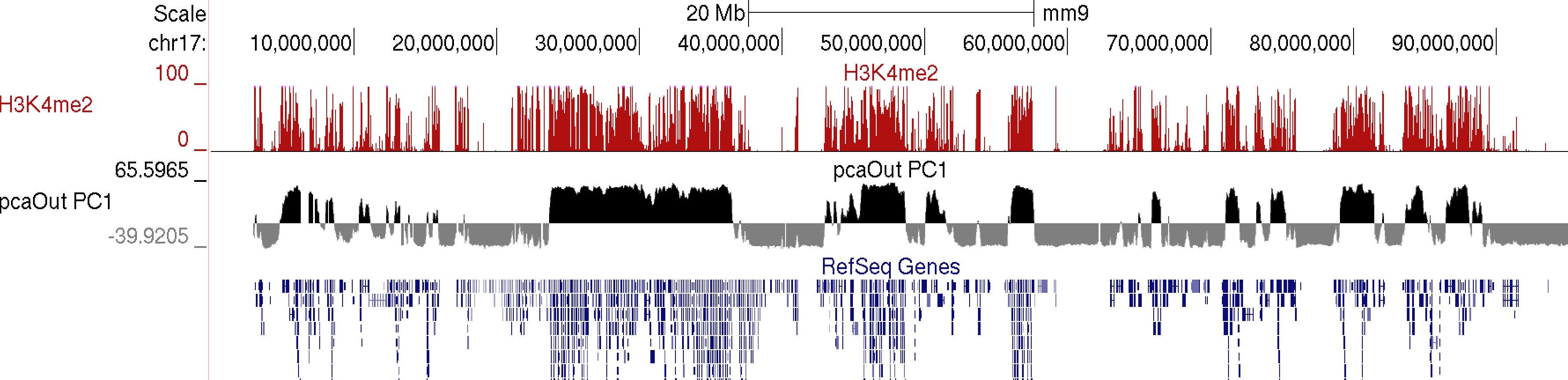
runHiCpca.pl <outputPrefix> <HiC Tag Directory> [options]

example: runHiCpca.pl pcaOut ES-HiC/ -res 50000 -cpu 4 -genome mm9

This command will produce two output files: *.PC1.txt and *.PC1.bedGraph (i.e. pcaOut.PC1.bedGraph).  The bedGraph file can be directly uploaded to UCSC and represents the coordinates of each region with respect to the first two principle components.  The txt file contains the same information in peak file format.  Below is an example of the output on chr17:



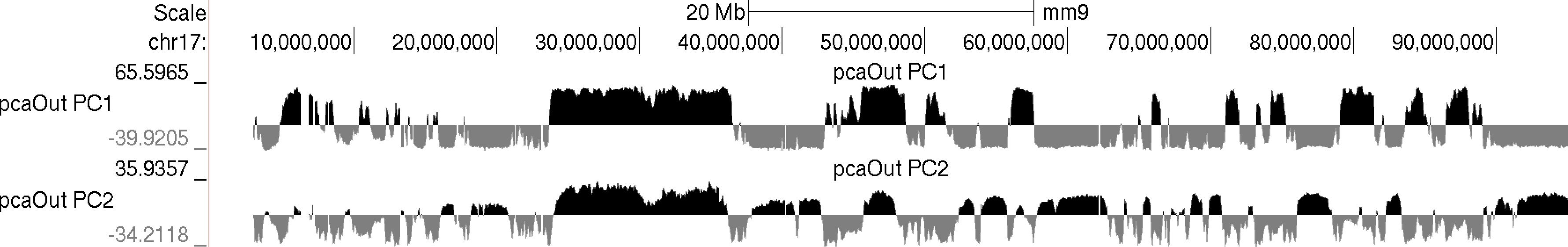
Usually the values for the first principal component (PC1) are the most informative.  These indicate the classification of each region of the chromosome with respect to the first component.  Normally, gene-rich regions with 'active' chromatin marks have similar PC1 values, while gene deserts tend to have the opposite.  You can also view additional principal components by changing the "-pc <#>" option.  The 2nd component (PC2) usually describes the the location along the chromosome (e.g. near telomere vs. centromere, or different chromosome arms).  The PC2 values tend look a lot like the PC1 values but usually "flip" along the length of the chromosome.  Their similarity is partly due to the fact that they are mathematically linked - Each principal component must be orthogonal to one another, so unless the first PC1 perfectly describes a feature of the data, other PCs might reflect the feature as well.  In the example below, PC1 and PC2 values are more similar for the first 40 Mb, and then they tend to be more opposite for the rest of the chromosome.




In general, this analysis tends to highlight the fact that the genome can be divided into two compartments, creating a "checkerboard" pattern, with positive PC1 regions reflecting "active/permissive" chromatin and negative PC1 regions indicative of "inactive/inert" chromatin

What does runHiCpca.pl do:

runHiCpca.pl is a wrapper script that will perform PCA analysis on each chromosome individually and combine all the results.  Below are each of the steps:

1. Check for the appropriate background model, create it if necessary.

2. For each chromosome:

- Generate normalized interaction matrix (analyzeHiC)
- Calculate correlation between the contact profiles from each region against each other region
- Using R, compute the principal components from the correlation matrix
- Output the values of reach region with respect to the first two principal components

3. If "seed" regions are provided, HOMER checks the overlap between active (and/or inactive) regions to decide if the coordinates should be multiplied by -1 to flip the signs.  HOMER will try to make it so regions in "active" zones are positive.  If no seed regions are used, but a genome is specified, HOMER will look for overlap with TSS to assign "active" vs. "inactive".

4. Concatenate results from all chromosomes, format, and print the output

runHiCpca.pl Options:

-pc <#> : Number of principal components to return (default: 1).

-res <#> : resolution of analysis (if it's too small, the program may take too long or use up too much memory).  A resolution of 25000 is about the limit for mammalian genomes, unless your computer is ridiculous... The sequencing depth and quality of an experiment may dictate which resolutions are possible.  If the PC1 values are very noisy you may need to increase the resolution size. Default: 50000

-superRes <#> : window size of analysis, should be equal to or larger than -res. Default: 100000.

-active <peak/BED file> : seed regions of "active" chromatin to use when assessing the proper sign of the PC1 results.

-inactive <peak/BED file> : seed regions of "inactive" chromatin to use when assessing the proper sign of the PC1 results.

-genome <genome> : If no seed regions are given, HOMER will get the TSS locations and treat them as "active" seeds.

-corrDepth <#> : Minimum number of expected reads per region to use when computing correlation (pools adjacent regions), default: 3

-std <#> : exclude regions with sequencing depth exceeding # std deviations, default: 4.  The idea here is to remove regions that may throw off the PCA calculation

-min <#> : exclude regions with sequencing depth less than this fraction of mean, default: 0.15.  The idea is to get rid of regions with low coverage that don't behave as well during the PCA analysis.

-rpath <path to R executable> : If "R" is not available through the $PATH variable (i.e. can't just type "R" to run R)

-cpu <#> : number of CPUs to use.  Memory consumption is also higher with more CPUs (work separated by chromosome).  Please note that if multiple CPUs are configured, the screen output will spew all over the place - just ignore it...

Directly Comparing Two Hi-C Experiments

PCA analysis is a useful tool for analyzing single Hi-C experiments.  However, comparing PC1 values between two experiments is a little dangerous.  PCA is an unbiased analysis of data, and while PC1 values usually correlated with "active" vs. "inactive" compartments, the precise qualitative nature of this association may differ slightly between experiments.  Because of this, it is recommended to directly compare the interaction profiles between experiments rather than simply looking at PC1 values.

One way to do this is to directly correlate the interaction profile of a locus in one experiment to the interaction profile of that same locus in another experiment.  If the locus tends to interact with similar regions in both Hi-C experiments, the correlation will be high.  If the locus interacts with different regions in the two experiments, the correlation will be low.  Note that this is NOT PCA analysis, cut a direct comparison between two experiments at each locus.  By default, this will compare the interaction profiles across each chromosomes (interchromosomal interactions are generally too sparse for this type of analysis)

To calculate the "correlation difference" between two experiments, use the getHiCcorrDiff.pl.  Below is how it's used:

getHiCcorrDiff.pl <outputPrefix> <HiC Tag Directory1> <HiC Tag Directory2> [options]

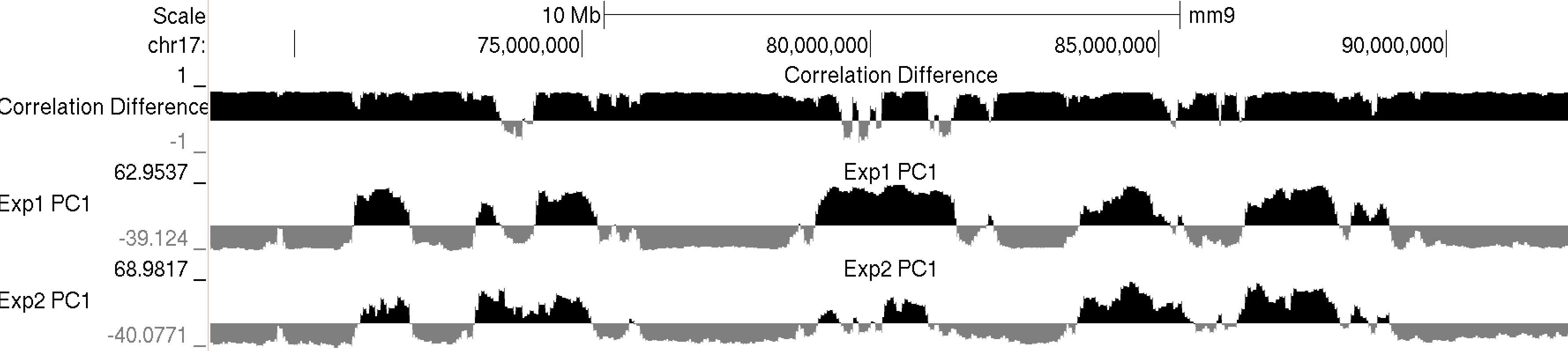
example: getHiCcorrDiff.pl out ES-HiC Bcell-HiC -cpu 8 -res 50000

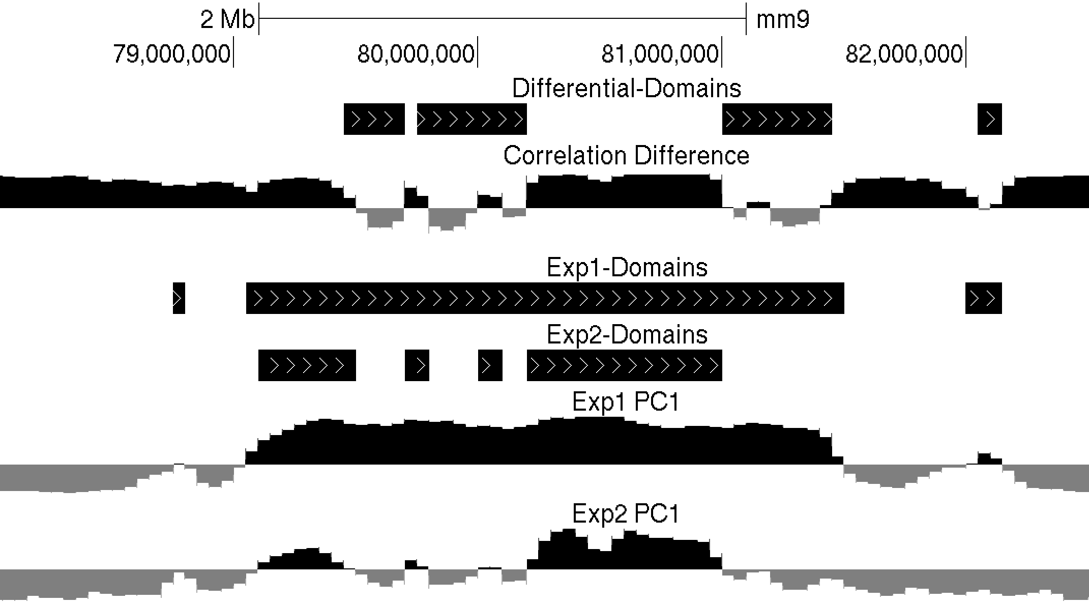
This program will produce two output files, much like runHiCpca.pl.  One is a bedGraph what can be loaded into the UCSC Genome Browser as a custom track.  The other is a peak file with the correlation information in the 6th column.  Below is an example of the corrDiff output loaded with the PC1 values from two experiments:

Additional Options for getHiCcorrDiff.pl:

-res <#> : resolution of analysis (if it's too small, the program may take too long or use up too much memory).  A resolution of 25000 is about the limit for mammalian genomes, unless your computer is ridiculous... The sequencing depth and quality of an experiment may dictate which resolutions are possible.  If the values are very noisy you may need to increase the resolution size. Default: 50000.

-superRes <#> : window size of analysis, should be equal to or larger than -res. Default: 100000.
               
-corrDepth <#> : Minimum number of expected reads per region to use when computing correlation (pools adjacent regions), default: 3

-std <#> : exclude regions with sequencing depth exceeding # std deviations, default: 4.  The idea here is to remove regions that may throw off the PCA calculation

-min <#> : exclude regions with sequencing depth less than this fraction of mean, default: 0.15.  The idea is to get rid of regions with low coverage that don't behave as well during the PCA analysis.

-maxDist <#> : By default, getHiCcorrDiff.pl compares each locus by looking at it's contact profile across the whole chromosome.  Setting this option will limit the profile comparison to the region +/- this distance from the locus (sort of like a 'local' correlation)

-cpu <#> : number of CPUs to use.  Memory consumption is also higher with more CPUs (work separated by chromosome).  Please note that if multiple CPUs are configured, the screen output will spew all over the place - just ignore it...

Downstream PC1 analysis

There are several ways to use HOMER to analyze PC1 values (or corrDiff values) with respect to other data.  Some are very general ways to manipulate bedGraphs, while others are very specialized to PC1 values (i.e. getDomains.pl).

Histograms/Quantifying PC1 values at genomic features

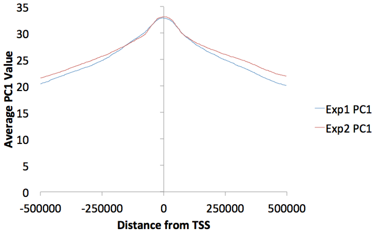
You can make histograms of PC1 values around areas of interest by using annotatePeaks.pl and the "-bedGraph" option.  Lets say you'd like to see the distribution of PC1 values around TSS. (alternatively you could look at PC1 values near ChIP-Seq peaks or other features)  Using the command below:

annotatePeaks.pl tss mm9 -size 1000000 -hist 1000 -bedGraph exp1.PC1.bedGraph exp2.PC1.bedGraph > output.histogram.txt

Opening the histogram output in Excel and graphing the "coverage" columns:

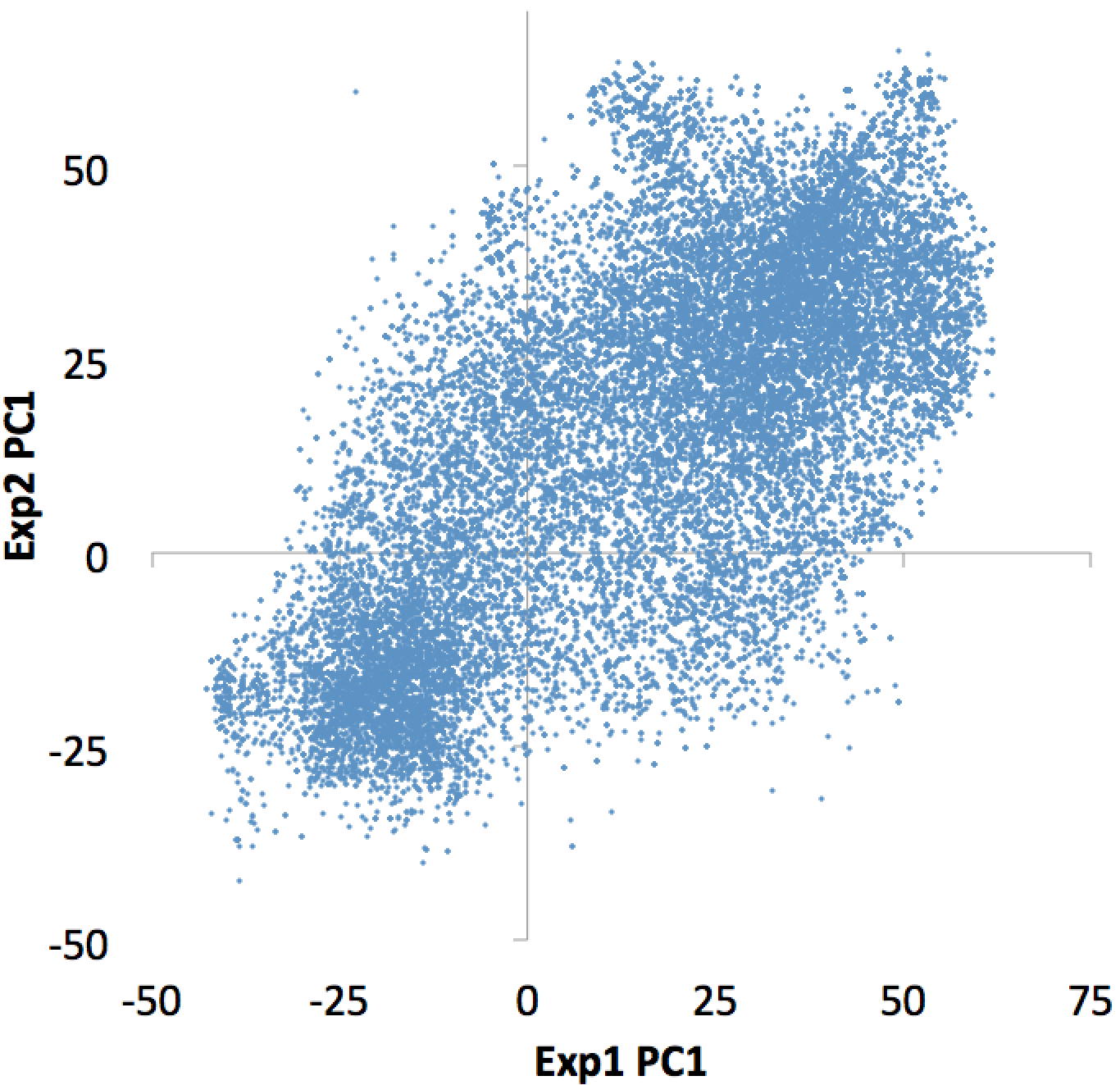
You can also omit the "-hist <#>" option and adjust the size from the annotatePeaks.pl command, and annotatePeaks.pl will instead quantify the PC1 values at each locus, which can be useful for classifying which TSS are in the 'active/permissive' compartment vs. which TSS are in the 'inactive/inert' compartment:

annotatePeaks.pl tss mm9 -size 1000 -bedGraph exp1.PC1.bedGraph exp2.PC1.bedGraph > output.table.txt

Opening this file with Excel:

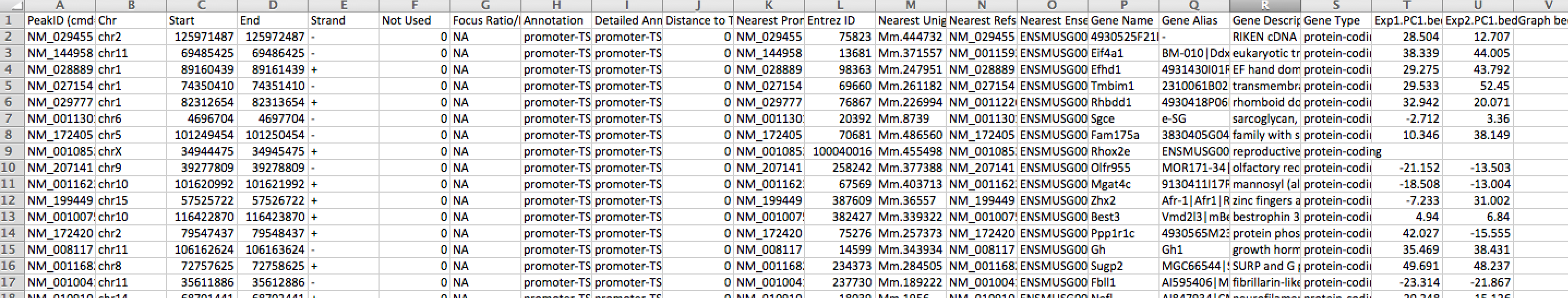
Plotting the bedGraph data columns as a scatter plot:

This file can also be used to figure out which individual TSS are changing the most, etc.  Similar operations could be performed on ChIP-Seq peaks or other features of interest.

Finding PC1 Based Compartments

Regions of continuous positive or negative PC1 values set the stage for identifying "compartments", in this case referring to linear regions of DNA that are in the "active/permissive" or "inactive/inert" compartments.  (This is a little different than the concept of topological domains reported in Dixon et al., which are more of a local phenomenon instead of a compartment association).  A custom tool is available in HOMER to help with this task named findHiCCompartments.pl.

Unlike the annotatePeaks.pl command avoid, findHiCCompartments.pl works on the *.PC1.txt files that are produced by runHiCpca.pl, not the *.PC1.bedGraph files.

To identify compartments, run the command:

findHiCCompartments.pl exp1.PC1.txt > compartments.txt

By default, this command will identify all regions that have a continuous positive PC1 value.  The output is a peak file that contains each of these regions, their average PC1 value across the region, and their length in the 6th and 7th columns, respectively.  To adjust the threshold used to call compartments, use the "-thresh <#>" option.  To identify regions with negative PC1 values, add the "-opp" option to the command.  Also, if you prefer to return compartments as the original sub-peaks (instead of stitching them together into a single, long peak), add the "-peaks" option.

Differential Compartments (i.e. Flipping)

The findHiCCompartments.pl command also has some built in support for identifying regions that change their compartment between experiments.  Two sources of information can be used to identify changes: the PC1 values from a second Hi-C experiment, and/or the correlation difference (i.e. getHiCcorrDiff.pl output) between two experiments.  If both options are used, the identified regions must pass both criterion.

-bg <PC1.txt file> : specify a background experiment's PC1 results.
-diff <#> : minimum difference between PC1 values to define region as different, default: 50

-corr <corrDiff.txt file> : specify a correlation difference file
-corrDiff <#> : maximum correlation for a region to be defined as different, default: 0.4

Below is an example of these files uploaded to the UCSC Genome Browser. NOTE: If UCSC complains that you chromsome coordinates exceed the end of the chromosome (could happen due to the resolution), run the command "removeOutOfBoundsReads.pl compartments.txt <genome> > compartments.new.txt" to adjust the coordinates at the end of the chromosome.

Clustering Regions Based on their Interactions

HOMER also offers more "direct" ways to group regions (most of these are experimental).  For now, it's recommended you stick to the PCA analysis from above, however, there may be situations where the routines below are more useful.

analyzeHiC has two types of clustering routines to help identify sets of regions that are "related" in 3D-space.  They are:

-cluster : Clustering of regions regardless of genomic locations (pure clustering based on interaction frequency)

-clusterFixed : Clustering of regions based on adjacent, linear, regions on the chromosome (for finding "linear domains")

The clustering is performed as hierarchical clustering, and the output is stored in files "out.cdt" and "out.gtr".  You can use Java Tree View to open the "out.cdt" file and view the clustering result.  From there you can select your own clusters if you like.  Selection of "-corr", "-logp" or "-simpleNorm" etc. during the command will cause those values to be used in the clustering instead of the default ("-norm"). 

To name the clustering output something other than "out", use "-o <filename>", which will use <filename> as the prefix for the clustering files instead of "out".

Example of -cluster

As an example, lets try clustering the normalized matrix of chr1 at 1 Mb resolution.  Using the command:

analyzeHiC ES-HiC/ -chr chr1 -res 1000000 -cluster > outputmatrix.txt

This produces several files, named out.cdt and out.gtr (and outputmatrix.txt, which we'll ignore).  Opening out.cdt with Java Tree View will give us:



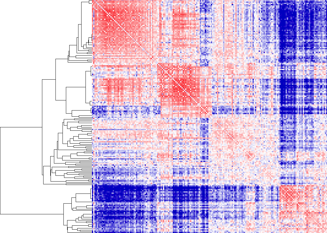
In this example, we allow "free clustering", and the algorithm will group together loci that are considered "close together" - in this case, loci whose interaction profiles have high interaction log2 ratios.  As you can see, there are essentially two groups.  To visualize which regions are in the groups, highlight the sub-tree of interest, and then export the list (under Export->Save List in Java Tree View).  HOMER contains a tool called cluster2bed.pl to allow you to visualize these clusters in the genome browser.  Run the following command on the saved list file (be default this is called "out_list.txt"):

cluster2bed.pl <cluster list> <#resolution> [# minimum to cluster size to keep]  > out2.bed
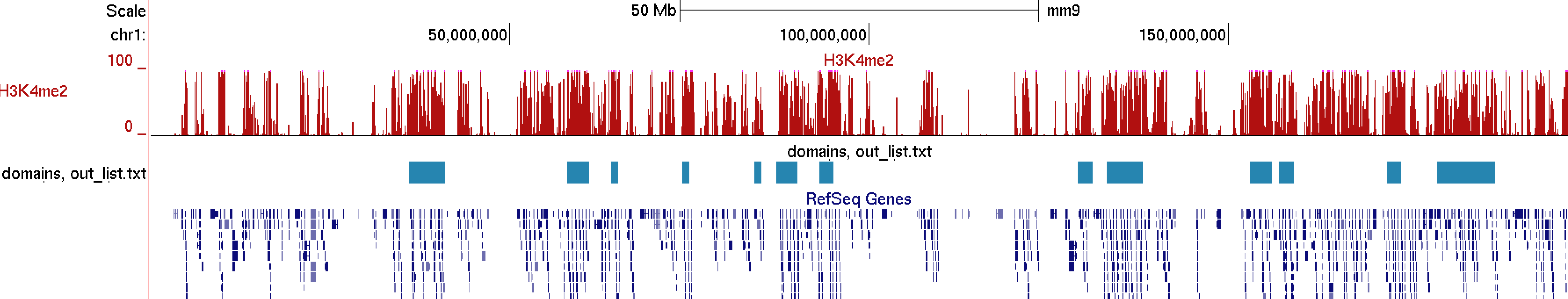
i.e. cluster2bed.pl out_list.txt 1000000  > out.bed

You can now upload the output file to the UCSC genome browser.  The 3rd option in the cluster2bed.pl command is optional, which will remove clusters containing only a couple regions (be default, it removes cluster containing fewer than 5% of the total).  Colors are randomly assigned to the clusters to help differentiate them.

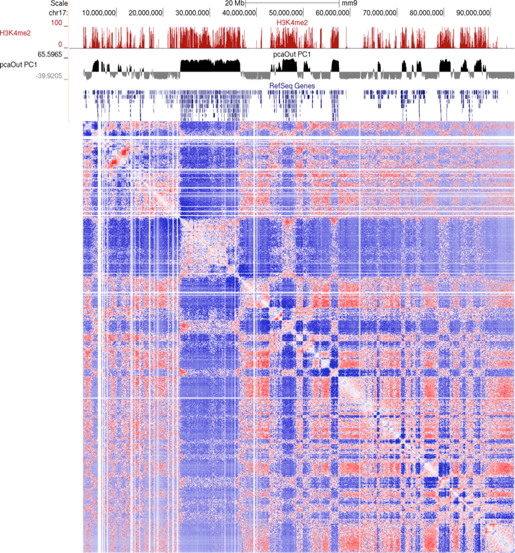
Visualizing these clusters in the UCSC genome browser along with H3K4me2 ChIP-Seq and the interaction matrix, you can see that the 2 major clusters from above correlate with H3K4me2 very nicely (would look better at higher resolution, say 100kb)

Example of -clusterFixed

As an example, lets try clustering again, this time using "fixed" clustering, which will force adjacent positions to be grouped.  Using the command:

analyzeHiC ES-HiC/ -chr chr1 -res 1000000 -clusterFixed > outputmatrix.txt

This produces the same basic output files as "-cluster", named out.cdt and out.gtr (and outputmatrix.txt, which we'll ignore).  Opening out.cdt with Java Tree View will give us:




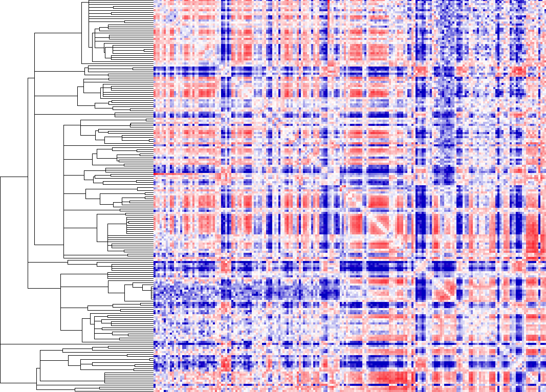
Here you'll notice that the heatmap look just as it would if you did not cluster the data.  The only difference is that it grouped regions together based on there similarity.  This can be useful for finding linear domains.  To extract domains from the clustering result, you must first choose a cutoff threshold to identify cluster (i.e. 0.5 - related to correlation) and use the "homerTools cluster" program, and then use the cluster2bed.pl tool to format for the UCSC Genome Browser:

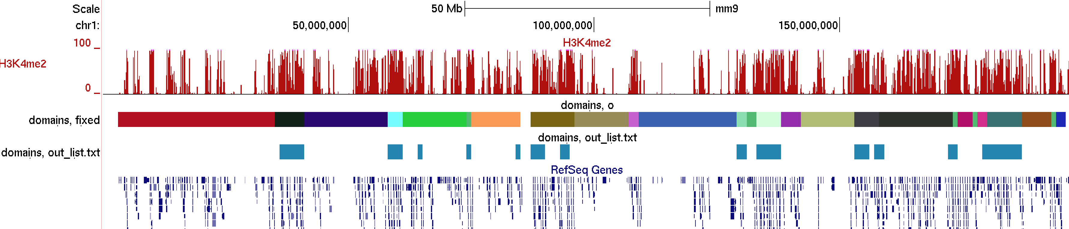
homerTools cluster -gtr out.gtr -thresh 0.5 > cluster.txt
cluster2bed.pl cluster.txt 1000000  > out.bed

Uploading this to the browser will give us:

Command Line Options for runHiCpca.pl

Command Line Options for getHiCcorrDiff.pl

Command Line Options for getDomains.pl