HOMER

Software for motif discovery and next-gen sequencing analysis

Hi-C Background Models: Normalizing Genomic Interactions for Linear Distance and Read Depth

Chromosome conformation capture (3C) and related technologies measure the frequency that two genomic fragments appear in close physical proximity (cross-linked in the same complex).  One of the goals when analyzing Hi-C data is to understand which loci in the genome tend to "interact" or "don't interact" in a biologically meaningful way.  Unfortunately, the total number Hi-C reads between any two loci is dependent on many factors, many of which need to be normalized before meaningful conclusions can be reached.

Primary Sources of Technical Bias in Hi-C Interaction Counts

Read depth per region: Since Hi-C is an unbiased assay of genomic structure, we expect to observe equal read coverage across the genome.  However, factors such as the ability to map reads uniquely (e.g. density of genomics repeats), the number of restriction sites, and genomic duplications/structural variation in the experimental sample will all influence the number of reads.

Linear distance between loci along the chromosome: If two loci are along the same polymer/chromosome of DNA, the loci are constrained with respect to one another independent of any specific structures adopted by the chromosome.  More to the point, loci closely spaced along a chromosome are almost guaranteed to be 'near' one another if for no other reason their maximal separation is the length of DNA between them.  As a result, closely spaced loci with have very high Hi-C read counts, regardless of their specific conformation.  This is generally true of all 3C-based assays.

Sequencing Bias: GC% bias, ligation preferences during library construction, normal sequencing problems.

Chromatin compaction: This source of bias isn't really an artifact as it reflects biologically meaningful configuration of chromatin fibers.  The idea is that different types of chromatin environments tend to "fold" in different ways, with heterochromatic/inactive/inert chromatin displaying a different average interaction frequencies as a function of distance than euchromatin/active/permissive regions.  However, when looking for specific interaction in a particular chromatin environment, it can be useful to understand the properties of your local region of DNA to help interpret what is meaningful or just normal for that type of chromatin environment.

Analyzing Hi-C data at different resolutions

Most Hi-C experiments to date are severely under-sequenced.  For example, there are approximately a million HindIII restriction sites in the genome.  If have 100 million [filtered] paired-end reads then we will only find 200 reads ends at each HindIII restriction fragment.  Since (in theory) each HindIII fragment may interact with each of the other fragments, we would observe on average 0.0002 reads connecting any two HindIII fragments in the genome.  In reality, most of these reads are between HindIII fragments that are within close proximity.  However, for many of the observed interactions, it is difficult to know if a single observed interaction is a significant event or simply noise.  Extremely high sequencing depth may help resolve this, but for the most part we are force to come up with more clever ways to analyze the data.

One of the simplest approaches is too analyze reads across large regions to boost the total number of reads considered.  This approach was used in the original Hi-C paper (Lieberman-Aiden et al.), and it remains a powerful strategy.  The resolution of the analysis is therefore an important consideration.

HOMER uses two (related) notions of resolution.  The first, "-res <#>" represents how frequent the genome is divided up into regions.  The second, the super resolution "-superRes <#>" (poorly named), represents how large the region is expanded when counting reads.  Usually the "-res <#>" should be smaller than the "-superRes <#>".  For example a res of 50000 and a superRes of 100000 would mean that HOMER will analyze the regions 0-50k, 50k-100k, 100k-150k etc., but at each region it will look at reads from a region the size of 100k, so it would look at reads from -25k-75k, 25k-125k, 75k-175k, etc.  This means HOMER will analyze data with overlapping windows.  The principle advantage to this strategy is that you don't penalize features that span boundaries.

Normalizing Hi-C Data

Since Hi-C analysis is an unbiased assay of nuclear topology, the expectation is that roughly equal numbers of Hi-C reads should originate from each region of equal size in the genome. If different numbers of Hi-C reads are observed, this is likely due to bias in mapping (e.g. repeats or duplicated genomic sequences in the region where no reads can be mapped), a variable number of restriction enzyme recognition sites (e.g. HindIII), or a technical artifact (i.e. inaccessibility of HindIII to DNA). For this reason, Hi-C reads between any two regions of a given size must be normalized for sequencing depth by dividing the total number of interaction reads that each region participates in. To calculate the expected Hi-C reads between two given regions, we use the following equation:

eij =(ni)(nj)/N

Where N is the total number of reads in the Hi-C experiment and n the total number of reads at each region i and j. This formulation assumes that each region has a uniform probability of interacting with any other region in the genome.

In addition to sequencing depth, it is also useful to normalize data based on the distance between interacting regions. The constrained proximity of regions along linear DNA is by far the strongest signal in Hi-C data, with regions found at close linear distances much more likely to generate Hi-C reads than regions located at large linear distances along the chromosome or located on separate chromosomes. By computing the average number of Hi-C reads as a function of distance and sequencing depth, read frequencies between specific regions can be reported relative to the average Hi-C read density for their linear distances to help reliably identify proximity relationships that are not simply a result of the general linear compaction along the DNA.

The general idea was to modify our calculation of the expected number of Hi-C reads between any two loci to account for both their linear distance and sequencing depth. However, this calculation requires that we know the true number of interaction reads originating from a given locus, and not the measured number of interaction reads. For example, if region A (mapped) is adjacent to a region B (repeat region, unmappable), the total number of Hi-C reads mapping to A will likely be much less than a scenario in which B can be mapped as well. This is particularly important of regions adjacent to regions that cannot be mapped where their linear proximity would predict a significant numbers of Hi-C reads to connect the regions. This phenomenon causes a problem when trying to estimate the expected number of reads connecting region A to another region C. Since the total number of reads mapped to A is less because of region B adjacent to A that cannot be mapped, we likely underestimate the number of Hi-C reads mapping A to C.

To account for this, we find the expected number of Hi-C reads can be found with the following equation:

eij = f(i-j) (n*i)(n*j)/N*

Where f is the expected frequency of Hi-C reads as a function of distance, N* is estimated total number of reads, and n* is the estimated total number of interaction reads at each region. The goal was to identify n*i such that the total number of expected reads at each region i as a function of sequencing depth and distance (Si=sum(eij)) is equal to the observed number of reads at each region ni. Because the expected number of reads in any given region depends on the number of reads in all other regions, the resulting nonlinear system is difficult to solve directly. Instead, a simple hill climbing optimization was used to estimate inferred total reads. To calculate the inferred number of reads at each region, the model for expected interactions above is used to compute the expected number of read totals for each region, using the actual numbers of interaction reads as the initial values. The difference between the observed number of reads and the expected number of reads is then used to scale the values for the estimated numbers of reads. This is computed for each region iteratively and repeated until the error between expected and observed Hi-C read totals per region is near zero.

Creating Hi-C Background Models

The primary/default normalization method attempts to normalize the data for sequencing depth and distance between loci.  To speed-up analysis, HOMER creates a "background model" that saves important parameters from normalization so that the background model only has to be computed once for a given resolution.  If you run HOMER routines with a certain resolution, HOMER will first check if the background model has been created (they are saved in the Hi-C Tag Directory).  If the appropriate background model is missing, HOMER will create it.  If for some reason you want to force the creation of a new model, use the "-force" option.

To create a background model, or force the creation of a new one, run analyzeHiC and use the "-bgonly" flag (this will create a background model and then quit):

analyzeHiC <HiC Tag Directory> -res <#> -bgonly -cpu <#>

i.e. analyzeHiC ES-HiC/ -res 100000 -bgonly -cpu 8

The output will be automatically saved in the file "<tag dir>/HiCbackground_#res_bp.txt" (i.e. "ES-HiC/HiCbackground_100000_bp.txt").

The background model creation process can be broken down into the following steps (example uses resolution of 100kb):

1. Divide the genome into putative regions (i.e. chr1:0-100kb, chr1:100kb-200kb, ... chrY:8900kb-9000kb)
2. Calculate the total read coverage in each region
3. Calculate the fraction of interactions spanning any given distance with respect to read depth
4. Optimize read count model to correctly assign expected interaction counts in regions with uneven sequencing depth
5. Calculate variation in interaction frequencies as a function of distance.

The process of background creation takes a while as it considers the interactions between every region at the size of the resolution.  This means breaking the genome into 100000 bp regions and examining how many interactions they have between one another.  For large resolutions, this isn't much of a problem, but for small resolutions the search space gets very large and the whole thing can take a long time.  As a result, the process is [slightly] parallel to speed things up (i.e. use "-cpu <#>" to use multiple processors).

Part of the reason this takes so long is that it takes care to consider the read coverage between each set of elements and take read depths at each location into account.  In the future, I would like to speed this up with some approximations that are probably 95% as good, just haven't gotten to it yet...

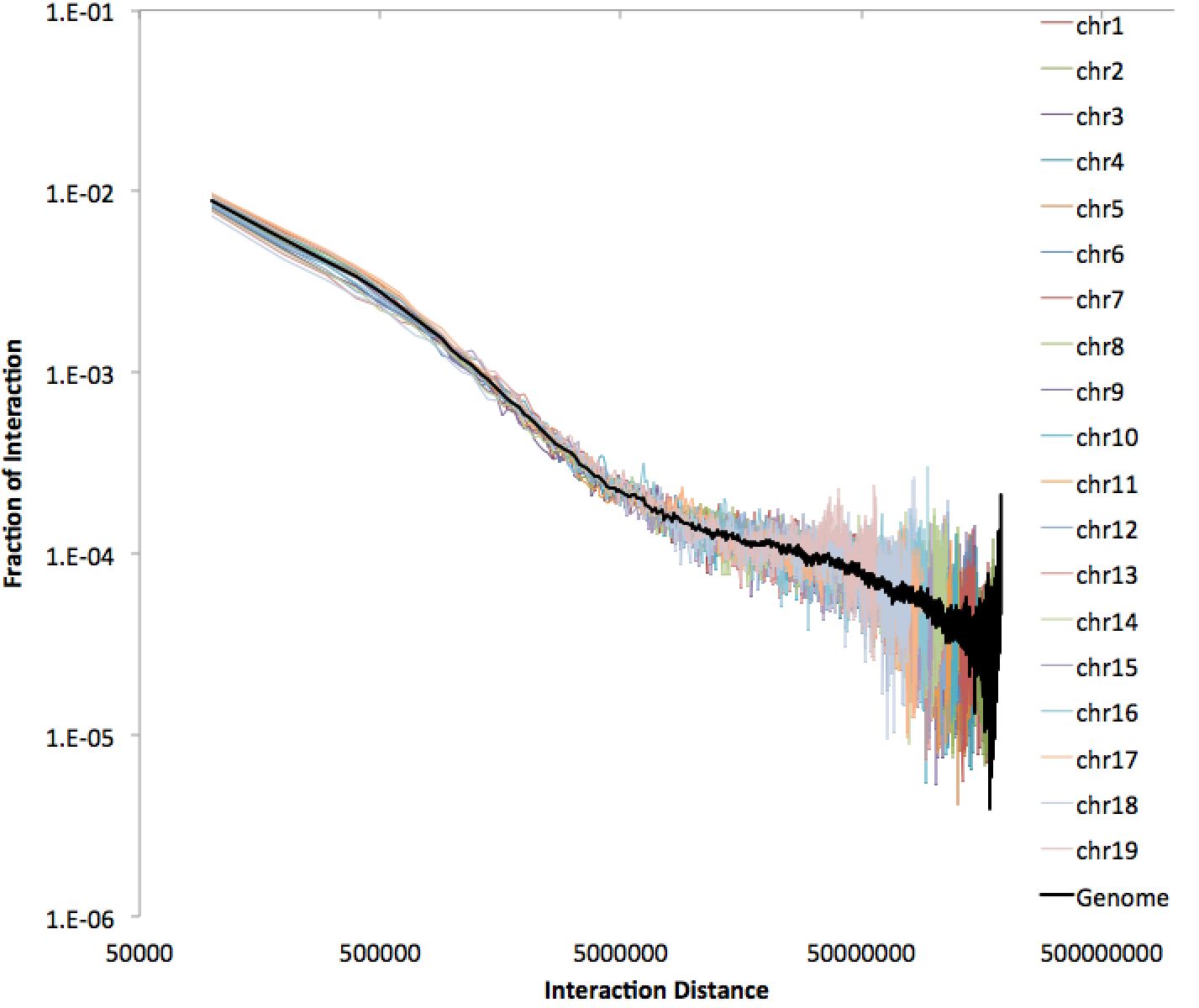
HiC Background Output File

There is a bunch of information in the file, including normalized interaction frequencies (both for the whole genome and for individual chromosomes).  The values, including interchromosomal ones, are meant to describe frequencies between regions, so they reflect the total number of such regions in the genome.  This file is interesting to graph in excel - for example, below is an example of a 100kb resolution file using a log-log plot on the interaction frequencies.

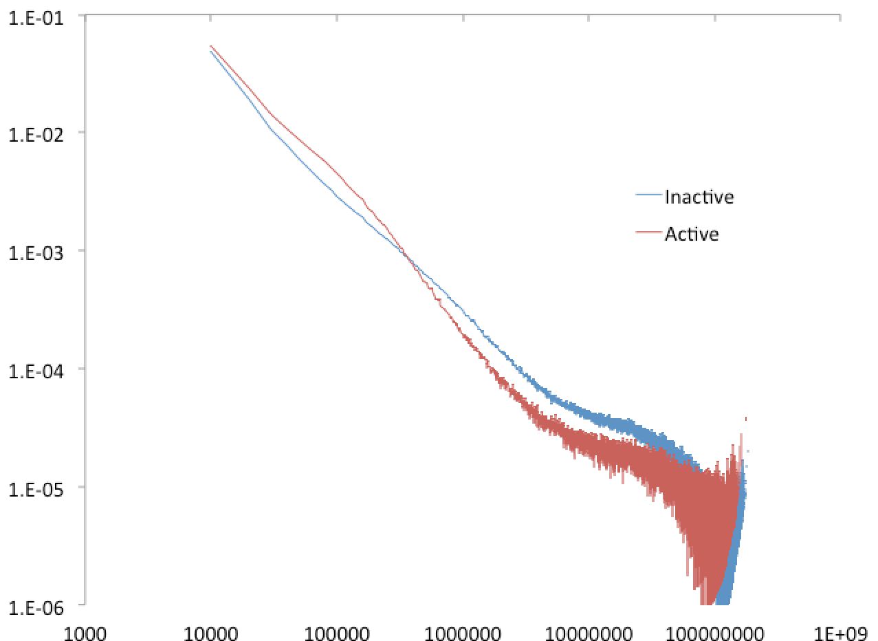
Creating Custom Background Models

By default, HOMER creates a background using the entire genome.  Sometimes you may want to understand the general properties in certain regions.  A classic example fro Lieberman-Aiden et al. is to look at the connectivity in "active" and "inactive" compartments.  To create a custom background model, use the option "-model <model output file>" to specify where to save the background model.  To use custom regions instead of the whole genome, create a peak file with the regions (i.e. active regions), and supply it as an argument with "-p <peak file>".

For example, lets say we have two peak files, one composed of active 100kb regions (with enrichment for H3K4me2) and another file with "inactive" regions.  Running the following commands:

analyzeHiC ES-HiC/ -createModel active.model.txt -p active.peaks.txt -vsGenome -res 100000 -cpu 8 -bgonly
analyzeHiC ES-HiC/ -createModel inactive.model.txt -p inactive.peaks.txt -vsGenome -res 100000 -cpu 8 -bgonly

We can open the "active.model.txt" and "inactive.model.txt" files, and compare their genome interaction profiles:

Custom background models can be used in downstream analysis by specifying the "-model <bgmodel.txt>".  For example, to use the "active.model.txt" from above, we would use:

analyzeHiC ES-HiC -model active.model.txt ...