
HOMER
Software for motif discovery and next-gen sequencing analysis
Quantifying Data and Motifs and Comparing Peaks/Regions
in the Genome
Homer contains a useful, all-in-one program for performing
peak annotation called annotatePeaks.pl.
In
addition
to
associating
peaks
with
nearby
genes,
annotatePeaks.pl can
perform Gene Ontology Analysis, genomic feature association
analysis (Genome Ontology), associate peaks with gene
expression data, calculate ChIP-Seq Tag densities from
different experiments, and find motif occurrences in
peaks. annotatePeaks.pl
can also be used to create histograms and heatmaps.
Description of the annotation functions are covered here, while quantification of
tags, motifs, histograms, etc. are covered below.Basic usage (see Annotation):
i.e. annotatePeaks.pl ERpeaks.txt hg18 > outputfile.txt
Everything packed into one program
Three primary options are available to specify types of data that can be processed by annotatePeaks.pl:
-m <motif file 1> [motif file 2] ...
-p <peak/BED file 1> [peak/BED file 2] ...
By default, these data types are processed relative to each peak/region provided in the primary input file. There are a bunch of options that help fine tune how each type of data is considered by the program covered below.
However, annotatePeaks.pl can take the same input data and do other things, such as make histograms and heatmaps, allowing you to explore the data in a different way.
Acceptable Input files
HOMER peak files should have at minimum 5 columns (separated by TABs, additional columns will be ignored):
- Column1: Unique Peak ID
- Column2: chromosome
- Column3: starting position
- Column4: ending position
- Column5: Strand (+/- or 0/1, where 0="+", 1="-")
- Column1: chromosome
- Column2: starting position
- Column3: ending position
- Column4: Unique Peak ID
- Column5: not used
- Column6: Strand (+/- or 0/1, where 0="+", 1="-")
Mac Users: If using a EXCEL to prepare input files, make sure to save files as a "Text (Windows)" if running MacOS - saving as "Tab delimited text" in Mac produces problems for the software. Otherwise, you can run the script "changeNewLine.pl <filename>" to convert the Mac-formatted text file to a Windows/Dos/Unix formatted text file.
If errors occur, it is likely that the file is not in the correct format, or the first column is not actually populated with unique identifiers.
TSS Mode
annotatePeaks.pl actually supports a variety of other specialty peaks depending on the genome. The most useful are 'tss' (described above), 'tts' (for transcription termination sites), and 'rna' (for peaks spanning whole gene bodies).
Specifying the Peak Size - the most important parameter
-size <#,#> : will perform analysis from # to # relative to peak center [example: -size -200,50]
-size given : will perform analysis on different sized peaks - size given by actual coordinates in peak/BED file [example: -size given]
For example, if you peaks are actually transcription start sites, you might want to specify "-size -500,100" to perform the analysis upstream -500 bp to +100 bp downstream. If your peaks/regions are actually "transcript" regions, specifying "-size given" will count reads along the entire transcript. If it doesn't make sense, watch Delta Force I and II back to back. That should numb the brain enough to get it.
Annotating Individual Peaks
Calculating ChIP-Seq Tag Densities across different experiments
output.txt, when opened in EXCEL, will look like this:
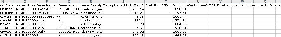
HOMER automatically normalizes each directory by the total number of mapped tags such that each directory contains 10 million tags. This total can be changed by specifying "-norm <#>" or by specifying "-noadj" or "-raw", both of which will skip this normalization step and report integer read counts.
The other new option available in HOMER is to output a rlog variance stabilized transformed data by specifying the "-rlog" option (R/DESeq2 must be installed on the system, see here). This is particularly useful if you want to use these values for downstream analysis such as clustering or PCA analysis. However, this is a potentially dangerous normalization if your data is from heterogeneous sources - in general this transformation is expecting data that is roughly similar across samples (i.e. all H3K27ac data).
The other important parameter when counting tags is to specify the size of the region you would like to count tags in with "-size <#>". For example, "-size 1000" will count tags in the 1kb region centered on each peak, while "-size 50" will count tags in the 50 bp region centered on the peak (default is 200). The number of tags is not normalized by the size of the region.
One last thing to keep in mind is that in order to fairly count tags, HOMER will automatically center tags based on their estimated ChIP-fragment lengths. This is can be overridden by specifying a fixed ChIP-fragment length using "-len <#>" or "-fragLength <#>". This is important to consider when trying to count RNA tags, or things such as 5' RNA CAGE/TSS-Seq, where you may want to specify "-len 0" so that HOMER doesn't try to move the tags before counting them.
HOMER can also quantify signal in bedGraph and WIG files using "-bedGraph <bedgraph file1> ..." and "-wig <wiggle file1> ...", respectively.
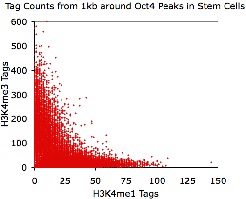
Making Scatter Plots
annotatePeaks.pl Oct4.peaks.txt mm8 -size 1000 -d H3K4me1-ChIP-Seq/ H3K4me3-ChIP-Seq/ > output.txt
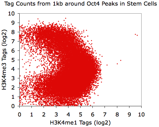
Using EXCEL to take the log(base 2) of the data:
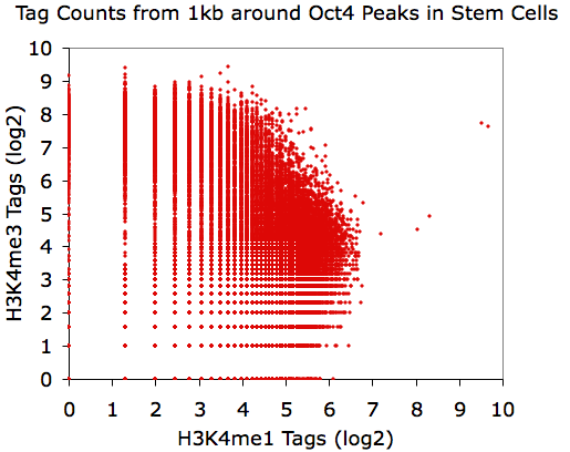
annotatePeaks.pl Oct4.peaks.txt mm8 -size 1000 -log -d H3K4me1-ChIP-Seq/ H3K4me3-ChIP-Seq/ > output.txt
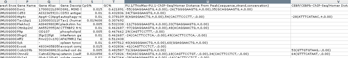
Finding instances of motifs near peaks
Opening output.txt with EXCEL:
There are also a bunch of motif specific options for specialized analysis:
"-nmotifs" (just report the total number of motifs per peak)
"-mscore" (report the maximum log-odds score of the motif in each peak)
"-rmrevopp <#>" (tries to avoid double counting reverse opposites within # bp)
"-mdist" (reports distance to closest motif)
"-fm <motif file 1> [motif file 2]" (list of motifs to filter out of results if found)
"-mfasta <filename>" (reports sites in a fasta file - for building new motifs)
"-mbed <filename>" (Output motif positions to a BED file to load at UCSC - see below)
"-matrix <filename>" (outputs a motif co-occurrence matrix with the p-value of co-occurrence assuming instance of each motif are independently distributed amongst the peaks)
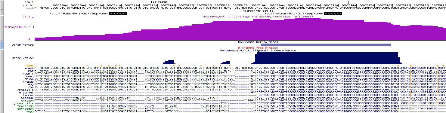
Visualizing Motif positions
in the UCSC Genome Browser
Finding the distance to other sets of Peaks
Creating Histograms from High-throughput Sequencing data
and Motifs
Basic usage:
i.e. annotatePeaks.pl ERpeaks.txt hg18 -size 6000 -hist 25 -d MCF7-H3K4me1/ MCF7-H3K4me2/ MCF7-H3K4me3/ > outputfile.txt
Running this command is very similar to creating annotated peak files - in fact, most of the data can be used to make both types of files - hence the reason for combining this functionality in the same command. Be default, HOMER normalizes the output histogram such that the resulting units are per bp per peak, on top of the standard total mapped tag normalization of 10 million tags.
Histograms of Tag
Directories:
Opening outputfile.txt with EXCEL, we see:
Graphing columns B and E while using column A for the x-coordinates, we get the following:
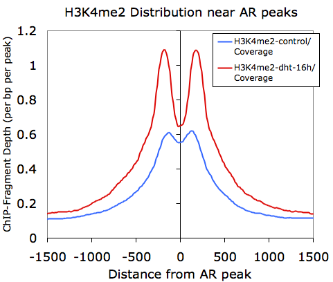
However, if we graph only the 5' and 3' tags that come from the H3K4me2-dht-16h directory (columns F and G):
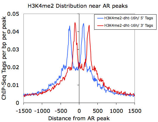
Here we can see how the 5' and 3' reads from the H3K4me2 marked nucleosomes are distributed near the AR sites.
Creating Meta-Gene Profiles
Homer (v4.8+) contains a tool called makeMetaGeneProfile.pl which automates the creation of 'meta-gene' profiles. What it does is automate the execution of annotatePeaks.pl several times for upstream, downstream and within the gene bodies of genes. You use the program in much the same way you use annotatePeaks.pl by passing tag directories, peak files, or motifs, but the controls for the histogram are slightly different:
makeMetaGeneProfile.pl <rna | peakfile> <genome> [histogram optoins] [annotatePeaks.pl options]
makeMetaGeneProfile.pl rna mm9 -p PU1.peaks.txt > output.txt
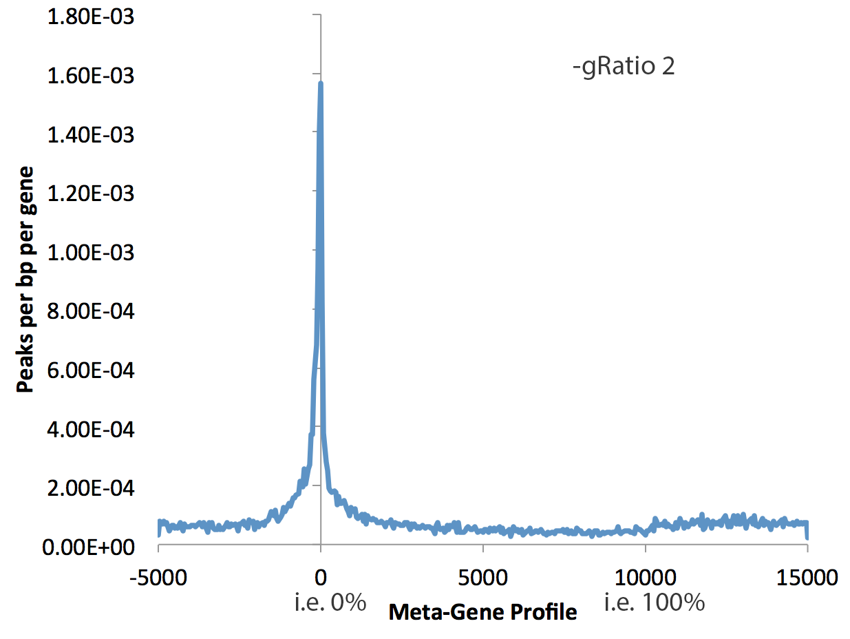
This can tool can be used with much more than gene bodies. The first argument can be an peak/BED file that you want. If you want to use RefSeq annotated gene bodies, use the key word "rna". By default, the program will quantify data from -5 kb to 0, then from 0% to 100%, then from 100% to +5kb. The following parameters control the behavior of makeMetaGeneProfile.pl:
- -min <#> : Minimum size of regions in peak file to use. This will remove peaks smaller than the given size, which is useful to avoid including small transcripts in the generation of meta-gene profiles. Default: 3000
- -max <#> : Maximum size of regions in peak file to use. Default: no max
- -gbin <#> : Number of bins in gene body, i.e. 100 means each bin is 1%. Default: 200
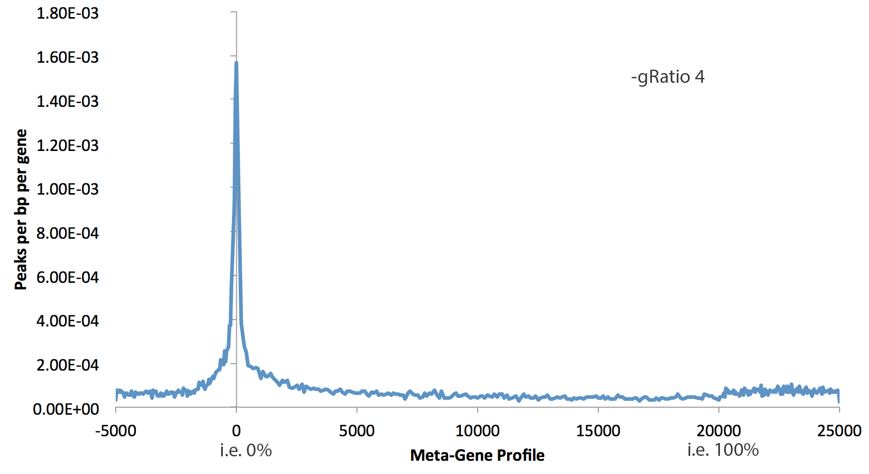
- -gRatio <#> : Controls the relative size of the plotted gene coverage relative to the the flanks (see examples below), Default: 2
- -bin <#> : size of bin in the flanks, default: 50
- -size <#> : size of flanks, default: 5000
Examples:
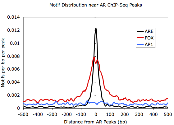
Histograms of Motif
Densities:
Graphing outputfile.txt with EXCEL:
Centering Peaks on Motifs
To center peaks on a motif, run annotatePeaks.pl with the following options:
i.e. annotatePeaks.pl ARpeaks.txt hg18r -size 200 -center are.motif > areCenteredPeaks.txt
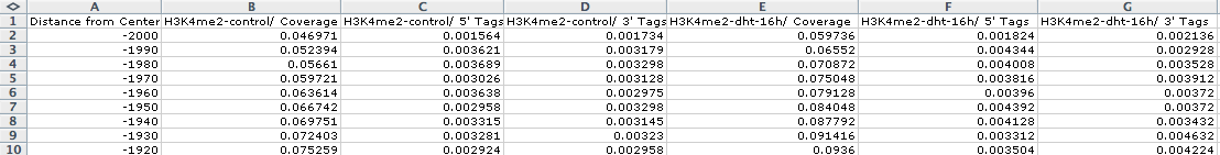
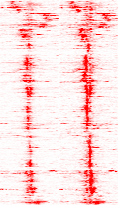
Creating Heatmaps from High-throughput Sequencing data
Basic usage (add "-ghist" when making a histogram):
i.e. annotatePeaks.pl ARpeaks.txt hg18 -size 6000 -hist 25 -ghist -d H3K4me2-control/ H3K4me2-dht-16h/ > outputfile.txt
Running this command is very similar to making histograms with annotatePeaks.pl. In fact, a heatmap isn't really all that different from a histogram - basically, instead of averaging all of the data from each peak, we keep data from each peak separate and visualize it all together in a heatmap. The key difference when making a heat map or a histogram is that you must add "-ghist" when making a heatmap.
Format of Data Matrix Output
File
After creating the file, I loaded into Cluster 3.0 to cluster and clustered the genes using "centered correlation" as the distance metric, then loaded that output into Java Tree View.
General Options to Control Data Analysis Behavior
-fragLength <#> (Fragment length, default=auto, might want to set to 0 for RNA)
-pc <#> (maximum number of tags to count per bp, default=0 [no maximum])
-cons (Retrieve conservation information for peaks/sites - creates new column for this information)
-CpG (Calculate CpG/GC content)
-norevopp (do not search for motifs on the opposite strand [works with -center too])
-norm <#> (normalize tags to this tag count, default=1e7, 0=average tag count in all directories)
Command line options for annotatePeaks.pl
Usage: annotatePeaks.pl <peak file | tss> <genome version> [additional options...]Available Genomes (required argument): (name,org,directory,default promoter set)
User defined annotation files (default is UCSC refGene annotation):
annotatePeaks.pl accepts GTF (gene transfer formatted) files to annotate positions relative
to custom annotations, such as those from de novo transcript discovery or Gencode.
-gtf <gtf format file> (-gff and -gff3 can work for those files, but GTF is better)
Peak vs. tss/tts/rna mode (works with custom GTF file):
If the first argument is "tss" (i.e. annotatePeaks.pl tss hg18 ...) then a TSS centric
analysis will be carried out. Tag counts and motifs will be found relative to the TSS.
(no position file needed) ["tts" now works too - e.g. 3' end of gene]
["rna" specifies gene bodies, will automaticall set "-size given"]
NOTE: The default TSS peak size is 4000 bp, i.e. +/- 2kb (change with -size option)
-list <gene id list> (subset of genes to perform analysis [unigene, gene id, accession,
probe, etc.], default = all promoters)
-cTSS <promoter position file i.e. peak file> (should be centered on TSS)
Primary Annotation Options:
-mask (Masked repeats, can also add 'r' to end of genome name)
-m <motif file 1> [motif file 2] ... (list of motifs to find in peaks)
-mscore (reports the highest log-odds score within the peak)
-nmotifs (reports the number of motifs per peak)
-mdist (reports distance to closest motif)
-mfasta <filename> (reports sites in a fasta file - for building new motifs)
-fm <motif file 1> [motif file 2] (list of motifs to filter from above)
-rmrevopp <#> (only count sites found within <#> on both strands once, i.e. palindromic)
-matrix <prefix> (outputs a motif co-occurrence files:
prefix.count.matrix.txt - number of peaks with motif co-occurrence
prefix.ratio.matrix.txt - ratio of observed vs. expected co-occurrence
prefix.logPvalue.matrix.txt - co-occurrence enrichment
prefix.stats.txt - table of pair-wise motif co-occurrence statistics
additional options:
-matrixMinDist <#> (minimum distance between motif pairs - to avoid overlap)
-matrixMaxDist <#> (maximum distance between motif pairs)
-mbed <filename> (Output motif positions to a BED file to load at UCSC (or -mpeak))
-d <tag directory 1> [tag directory 2] ... (list of experiment directories to show
tag counts for) NOTE: -dfile <file> where file is a list of directories in first column
-bedGraph <bedGraph file 1> [bedGraph file 2] ... (read coverage counts from bedGraph files)
-wig <wiggle file 1> [wiggle file 2] ... (read coverage counts from wiggle files)
-p <peak file> [peak file 2] ... (to find nearest peaks)
-pdist to report only distance (-pdist2 gives directional distance)
-pcount to report number of peaks within region
-vcf <VCF file> (annotate peaks with genetic variation infomation, one col per individual)
-editDistance (Computes the # bp changes relative to reference)
-individuals <name1> [name2] ... (restrict analysis to these individuals)
-gene <data file> ... (Adds additional data to result based on the closest gene.
This is useful for adding gene expression data. The file must have a header,
and the first column must be a GeneID, Accession number, etc. If the peak
cannot be mapped to data in the file then the entry will be left empty.
-go <output directory> (perform GO analysis using genes near peaks)
-genomeOntology <output directory> (perform genomeOntology analysis on peaks)
-gsize <#> (Genome size for genomeOntology analysis, default: 2e9)
Annotation vs. Histogram mode:
-hist <bin size in bp> (i.e 1, 2, 5, 10, 20, 50, 100 etc.)
The -hist option can be used to generate histograms of position dependent features relative
to the center of peaks. This is primarily meant to be used with -d and -m options to map
distribution of motifs and ChIP-Seq tags. For ChIP-Seq peaks for a Transcription factor
you might want to use the -center option (below) to center peaks on the known motif
** If using "-size given", histogram will be scaled to each region (i.e. 0-100%), with
the -hist parameter being the number of bins to divide each region into.
Histogram Mode specific Options:
-nuc (calculated mononucleotide frequencies at each position,
Will report by default if extracting sequence for other purposes like motifs)
-di (calculated dinucleotide frequencies at each position)
-histNorm <#> (normalize the total tag count for each region to 1, where <#> is the
minimum tag total per region - use to avoid tag spikes from low coverage
-ghist (outputs profiles for each gene, for peak shape clustering)
-rm <#> (remove occurrences of same motif that occur within # bp)
Peak Centering: (other options are ignored)
-center <motif file> (This will re-center peaks on the specified motif, or remove peak
if there is no motif in the peak. ONLY recentering will be performed, and all other
options will be ignored. This will output a new peak file that can then be reanalyzed
to reveal fine-grain structure in peaks (It is advised to use -size < 200) with this
to keep peaks from moving too far (-mirror flips the position)
-multi (returns genomic positions of all sites instead of just the closest to center)
Advanced Options:
-len <#> / -fragLength <#> (Fragment length, default=auto, might want to set to 0 for RNA)
-size <#> (Peak size[from center of peak], default=inferred from peak file)
-size #,# (i.e. -size -10,50 count tags from -10 bp to +50 bp from center)
-size "given" (count tags etc. using the actual regions - for variable length regions)
-log (output tag counts as log2(x+1+rand) values - for scatter plots)
-sqrt (output tag counts as sqrt(x+rand) values - for scatter plots)
-strand <+|-|both> (Count tags on specific strands relative to peak, default: both)
-pc <#> (maximum number of tags to count per bp, default=0 [no maximum])
-cons (Retrieve conservation information for peaks/sites)
-CpG (Calculate CpG/GC content)
-ratio (process tag values as ratios - i.e. chip-seq, or mCpG/CpG)
-nfr (report nuclesome free region scores instead of tag counts, also -nfrSize <#>)
-norevopp (do not search for motifs on the opposite strand [works with -center too])
-noadj (do not adjust the tag counts based on total tags sequenced)
-norm <#> (normalize tags to this tag count, default=1e7, 0=average tag count in all directories)
-pdist (only report distance to nearest peak using -p, not peak name)
-map <mapping file> (mapping between peak IDs and promoter IDs, overrides closest assignment)
-noann, -nogene (skip genome annotation step, skip TSS annotation)
-homer1/-homer2 (by default, the new version of homer [-homer2] is used for finding motifs)

Can't figure something out? Questions, comments, concerns, or other feedback:
cbenner@ucsd.edu