HOMER
Software for motif discovery and next-gen sequencing analysis
Annotating Regions in the Genome (annotatePeaks.pl)
Homer contains a useful, all-in-one program for performing
peak annotation called annotatePeaks.pl.
In
addition
to
associating
peaks
with
nearby
genes,
annotatePeaks.pl can
perform Gene Ontology Analysis, genomic feature association
analysis (Genome Ontology), associate peaks with gene
expression data, calculate ChIP-Seq Tag densities from
different experiments, and find motif occurrences in
peaks. annotatePeaks.pl
can also be used to create histograms and heatmaps.
Description of the annotation functions are covered below,
while quantification of tags, motifs, histograms, etc. are
covered here.Basic usage:
annotatePeaks.pl <peak/BED file>
<genome> > <output file>
i.e. annotatePeaks.pl ERpeaks.txt hg18 > outputfile.txt
i.e. annotatePeaks.pl ERpeaks.txt hg18 > outputfile.txt
The first two arguments, the
<peak file> and <genome>, are required, and must be the
first two arguments. Other optional command line
arguments can be placed in any order after the first
two. By default, annotatePeaks.pl
prints the program output to stdout, which can be captured in a file
by appending " > filename" to the command. With
most uses of annotatePeaks.pl,
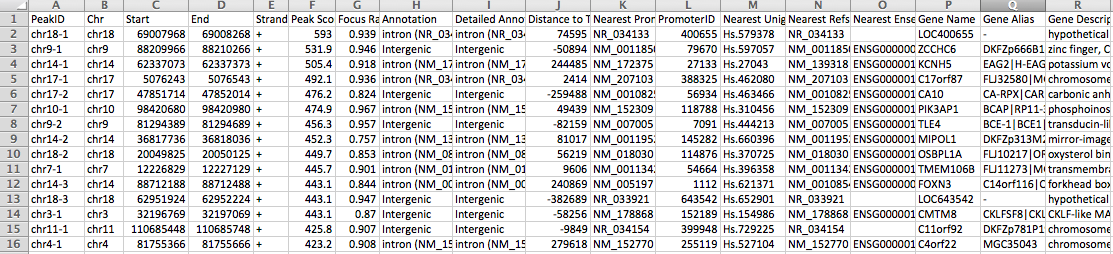
the output is a data table that is meant to be opened with
EXCEL or similar program. An example of the output
can been seen below:
Acceptable Input files
annotatePeaks.pl accepts HOMER peak files
or BED files:
HOMER peak files should have at minimum 5 columns (separated by TABs, additional columns will be ignored):
HOMER peak files should have at minimum 5 columns (separated by TABs, additional columns will be ignored):
- Column1: Unique Peak ID
- Column2: chromosome
- Column3: starting position
- Column4: ending position
- Column5: Strand (+/- or 0/1, where 0="+", 1="-")
BED files should have at
minimum 6 columns (separated by TABs, additional columns
will be ignored)
- Column1: chromosome
- Column2: starting position
- Column3: ending position
- Column4: Unique Peak ID
- Column5: not used
- Column6: Strand (+/- or 0/1, where 0="+", 1="-")
In theory, HOMER will accept
BED files with only 4 columns (+/- in the 4th column), and
files without unique IDs, but this is NOT recommended.
Mac Users: If using a EXCEL to prepare input files, make sure to save files as a "Text (Windows)" if running MacOS - saving as "Tab delimited text" in Mac produces problems for the software. Otherwise, you can run the script "changeNewLine.pl <filename>" to convert the Mac-formatted text file to a Windows/Dos/Unix formatted text file.
If errors occur, it is likely that the file is not in the correct format, or the first column is not actually populated with unique identifiers.
How Basic Annotation Works
The process of annotating
peaks/regions is divided into two primary parts. The
first determines the distance to the nearest TSS and
assigns the peak to that gene. The second determines
the genomic annotation of the region occupied by the
center of the peak/region.
Distance to the nearest TSS
Distance to the nearest TSS
By default,
annotatePeaks.pl loads a file in the "/path-to-homer/data/genomes/<genome>/<genome>.tss"
that contains the positions of RefSeq transcription
start sites. It uses these positions to determine
the closest TSS, reporting the distance (negative values
mean upstream of the TSS, positive values mean
downstream), and various annotation information linked
to each locus including alternative identifiers
(unigene, entrez gene, ensembl, gene symbol etc.).
This information is also used to link gene-specific
information (see below) to a peak/region, such as gene
expression.
Genomic Annotation
Calculating Peak Enrichment for Genomic Annotations
To annotate the location
of a given peak in terms of important genomic features,
annotatePeaks.pl
calls a separate program (assignGenomeAnnotation) to efficiently
assign peaks to one of millions of possible annotations
genome wide. Two types of output are
provided. The first is "Basic Annotation" that
includes whether a peak is in the TSS (transcription
start site), TTS (transcription termination site), Exon
(Coding), 5' UTR Exon, 3' UTR Exon, Intronic, or
Intergenic, which are common annotations that many
researchers are interested in. A second round of
"Detailed Annotation" also includes more detailed
annotation, considering repeat elements and CpG
islands. Since some annotation overlap, a priority
is assign based on the following (in case of ties it's
random [i.e. if there are two overlapping repeat element
annotations]):
Although HOMER doesn't allow you to explicitly change the definition of the region that is the TSS (-1kb to +100bp), you can "do it yourself" by sorting the annotation output in EXCEL by the "Distance to nearest TSS" column, and selecting those within the range you are interested in.
- TSS (by default defined from -1kb to +100bp)
- TTS (by default defined from -100 bp to +1kb)
- CDS Exons
- 5' UTR Exons
- 3' UTR Exons
- **CpG Islands
- **Repeats
- Introns
- Intergenic
Although HOMER doesn't allow you to explicitly change the definition of the region that is the TSS (-1kb to +100bp), you can "do it yourself" by sorting the annotation output in EXCEL by the "Distance to nearest TSS" column, and selecting those within the range you are interested in.
Calculating Peak Enrichment for Genomic Annotations
In addition to assigning genomic annotations to each peak, this program will also output the relative enrichment of your peaks in each set of genomic annotations (i.e. enrichment of the peaks in promoter regions, exons, CpG Islands, etc.). This calculation is performed by first identifying the fraction of the annotated genome assigned to each annotation. This is used to establish the expected distribution of peaks for each annotation. This is then compared to the observed fraction of peaks assigned to each annotation, using the binomial distribution to assign a significance p-value. To avoid divide by zero errors, annotations not assigned to a peak are given a pseudo count of one minus the expected fraction of peaks for that annotation when calculating the observed vs. expected log2 ratios and p-values.
Using Custom Annotations
Custom Gene Annotation Definition using GTF files
RefSeq doesn't do it for
everyone. There are many other quality gene
annotations out there, including UCSC genes, Ensembl,
and Gencode to name a couple. Even more important,
as RNA-Seq methods develop, the locations of exons etc.
can be defined based on your own experimental RNA data
rather than using a static database to define
transcripts. You can download GTF files for
various gene definitions from the UCSC Genome Browser in
the "Table
Browser" section. Custom GTF files can be
created from RNA-Seq data using tools like Cufflinks.
HOMER can process GTF (Gene Transfer Format) files and use them for annotation purposes ("-gtf <gtf filename>"). If a GTF file is specified, HOMER will parse it and use the TSS from the GTF file for determining the distance to the nearest TSS. It will also use the GTF file's definition of TSS/TTS/exons/Introns for Basic Genome Annotation. The original HOMER annotation files are still used for the "Detailed Annotation" since the repeats will not be define in the GTF files.
HOMER can process GTF (Gene Transfer Format) files and use them for annotation purposes ("-gtf <gtf filename>"). If a GTF file is specified, HOMER will parse it and use the TSS from the GTF file for determining the distance to the nearest TSS. It will also use the GTF file's definition of TSS/TTS/exons/Introns for Basic Genome Annotation. The original HOMER annotation files are still used for the "Detailed Annotation" since the repeats will not be define in the GTF files.
i.e. annotatePeaks.pl
ERpeaks.txt hg18 -gtf gencode.gtf >
outputfile.txt
HOMER will try it's best to take the "transcript_id" from the GTF definition and translate it into a known gene identifier. If it can't match it to a known gene, many of the annotation columns corresponding to Unigene etc. will be empty.
HOMER can also work with GFF and GFF3 files - to a degree. The problem with these is that the formats do not have the same strict naming convention enforced in GTF files. To use them, substitute "-gtf <GTF file>" with "-gff <GFF file>" or "-gff3 <GFF3 file>"
Custom Promoter Locations
By default, annotatePeaks.pl assigns
peaks to the nearest TSS. If you have a custom
peak/pos file of these locations, you can supply that
with the option "-cTSS
<peak/pos file>". This will
override the default, which is RefSeq TSS.
NOTE: For extreme control over annotations and use of the '-ann' option, check out the advanced annotation page.
Using Custom Genomes/Annotations
For organisms with
relatively incomplete genomes, annotatePeaks.pl can still
provide some functionality. If the genome is not
available as a pre-configured genome in HOMER, then you
can supply the path to the full genome FASTA file or path
to directory containing chromsome FASTA files as the 2nd
argument. For example, lets say you were sequencing
the
banana slug genome, and had downloaded the current
draft of the genome into the file "bananaSlug.fa".
You could then run annotatePeaks.pl like this:
If no genome sequence is available, you can also specify "none":
You may also find a custom annotation file for the organism, such as banana_slug_genes.gtf, or banana_slug_genes.gff from the community website. This can then be used to help annotate your data:
In the case of custom genomes, HOMER will not be able to convert gene IDs to names - you may have to do this yourself, but many of the other features, including motif finding etc., are available as long as you have the sequence.
annotatePeaks.pl chip-seq-peaks.txt
bananaSlug.fa > output.txt
If no genome sequence is available, you can also specify "none":
annotatePeaks.pl chip-seq-peaks.txt none >
output.txt
You may also find a custom annotation file for the organism, such as banana_slug_genes.gtf, or banana_slug_genes.gff from the community website. This can then be used to help annotate your data:
annotatePeaks.pl chip-seq-peaks.txt
bananaSlug.fa -gtf banana_slug_genes.gtf >
output.txt
or
annotatePeaks.pl chip-seq-peaks.txt bananaSlug.fa -gff banana_slug_genes.gff > output.txt
or
annotatePeaks.pl chip-seq-peaks.txt bananaSlug.fa -gff banana_slug_genes.gff > output.txt
In the case of custom genomes, HOMER will not be able to convert gene IDs to names - you may have to do this yourself, but many of the other features, including motif finding etc., are available as long as you have the sequence.
NOTE: For extreme control over annotations and use of the '-ann' option, check out the advanced annotation page.
Basic Annotation File Output
Description of Columns:
- Peak ID
- Chromosome
- Peak start position
- Peak end position
- Strand
- Peak Score
- FDR/Peak Focus Ratio/Region Size
- Annotation (i.e. Exon, Intron, ...)
- Detailed Annotation (Exon, Intron etc. + CpG Islands,
repeats, etc.)
- Distance to nearest RefSeq TSS
- Nearest TSS: Native ID of annotation file
- Nearest TSS: Entrez Gene ID
- Nearest TSS: Unigene ID
- Nearest TSS: RefSeq ID
- Nearest TSS: Ensembl ID
- Nearest TSS: Gene Symbol
- Nearest TSS: Gene Aliases
- Nearest TSS: Gene description
- Additional columns depend on options selected when running the program.
As of now, basic annotation
is based on alignments of RefSeq transcripts to the UCSC
hosted genomes.
Adding Gene Expression Data
annotatePeaks.pl can add gene-specific
information to peaks based on each peak's nearest
annotated TSS. To add gene expression or other data
types, first create a gene data file (tab delimited text
file) where the first column contains gene identifiers,
and the first row is a header describing the contents of
each column. In principle, the contents of these
columns doesn't mater. To add this information to
the annotation result, use the "-gene <gene data file>".
annotation.pl <peak
file> <genome> -gene <gene data file>
> output.txt
For peaks that are near
genes with associated data in the "gene data file", this
data will be appended to the end of the row for each peak.
Peak Annotation Enrichment
Gene Ontology Analysis of Associated Genes
annotatePeaks.pl offers two types of
annotation enrichment analysis. The first is based
on Gene Ontology classifications for genes. The
idea is that your regions (i.e. ChIP-Seq peaks) might be
preferentially found near genes with specific biological
functions. By specifying "-go <GO output
directory>", HOMER will take the list of
genes associated with your regions and search for
enriched functional categories, placing the output in
the indicated directory. This is just like looking
for GO enrichment in a set of regulated genes (covered in greater detail
here).
There are some caveats to this type of analysis - for example, some genes are simply more likely to be considered in the analysis if there are isolated along the genome where they are likely to be the "closest gene" for peaks in the region. But... since gene density roughly correlates with transcription factor density, it works itself out to some degree. Other tools, such as GREAT attempt to deal with this problem to some degree, and are worth trying. My experience is that the results are not that different once you factor in the fact that most other tools use "GO slims".
There are some caveats to this type of analysis - for example, some genes are simply more likely to be considered in the analysis if there are isolated along the genome where they are likely to be the "closest gene" for peaks in the region. But... since gene density roughly correlates with transcription factor density, it works itself out to some degree. Other tools, such as GREAT attempt to deal with this problem to some degree, and are worth trying. My experience is that the results are not that different once you factor in the fact that most other tools use "GO slims".
Genome Ontology: Looking for Enriched Genomic
Annotations
The Genome Ontology
looks for enrichment of various genomic annotations in
your list of peaks/regions. Just as the Gene
Ontology contains groups of genes sharing a biological
function, the Genome Ontology contains groups of genomic
regions sharing an annotation, such as TSS, or LINE
repeats, coding exons, Transcription factor peaks,
etc. To run the Genome Ontology, add the option "-genomeOntology <output
directory>". A much more detailed
description of the Genome Ontology will be available here (coming
soon).
Command line options for annotatePeaks.pl
Usage: annotatePeaks.pl <peak file | tss> <genome version> [additional options...]Available Genomes (required argument): (name,org,directory,default promoter set)
User defined annotation files (default is UCSC refGene annotation):
annotatePeaks.pl accepts GTF (gene transfer formatted) files to annotate positions relative
to custom annotations, such as those from de novo transcript discovery or Gencode.
-gtf <gtf format file> (-gff and -gff3 can work for those files, but GTF is better)
Peak vs. tss/tts/rna mode (works with custom GTF file):
If the first argument is "tss" (i.e. annotatePeaks.pl tss hg18 ...) then a TSS centric
analysis will be carried out. Tag counts and motifs will be found relative to the TSS.
(no position file needed) ["tts" now works too - e.g. 3' end of gene]
["rna" specifies gene bodies, will automaticall set "-size given"]
NOTE: The default TSS peak size is 4000 bp, i.e. +/- 2kb (change with -size option)
-list <gene id list> (subset of genes to perform analysis [unigene, gene id, accession,
probe, etc.], default = all promoters)
-cTSS <promoter position file i.e. peak file> (should be centered on TSS)
Primary Annotation Options:
-mask (Masked repeats, can also add 'r' to end of genome name)
-m <motif file 1> [motif file 2] ... (list of motifs to find in peaks)
-mscore (reports the highest log-odds score within the peak)
-nmotifs (reports the number of motifs per peak)
-mdist (reports distance to closest motif)
-mfasta <filename> (reports sites in a fasta file - for building new motifs)
-fm <motif file 1> [motif file 2] (list of motifs to filter from above)
-rmrevopp <#> (only count sites found within <#> on both strands once, i.e. palindromic)
-matrix <prefix> (outputs a motif co-occurrence files:
prefix.count.matrix.txt - number of peaks with motif co-occurrence
prefix.ratio.matrix.txt - ratio of observed vs. expected co-occurrence
prefix.logPvalue.matrix.txt - co-occurrence enrichment
prefix.stats.txt - table of pair-wise motif co-occurrence statistics
additional options:
-matrixMinDist <#> (minimum distance between motif pairs - to avoid overlap)
-matrixMaxDist <#> (maximum distance between motif pairs)
-mbed <filename> (Output motif positions to a BED file to load at UCSC (or -mpeak))
-d <tag directory 1> [tag directory 2] ... (list of experiment directories to show
tag counts for) NOTE: -dfile <file> where file is a list of directories in first column
-bedGraph <bedGraph file 1> [bedGraph file 2] ... (read coverage counts from bedGraph files)
-wig <wiggle file 1> [wiggle file 2] ... (read coverage counts from wiggle files)
-p <peak file> [peak file 2] ... (to find nearest peaks)
-pdist to report only distance (-pdist2 gives directional distance)
-pcount to report number of peaks within region
-vcf <VCF file> (annotate peaks with genetic variation infomation, one col per individual)
-editDistance (Computes the # bp changes relative to reference)
-individuals <name1> [name2] ... (restrict analysis to these individuals)
-gene <data file> ... (Adds additional data to result based on the closest gene.
This is useful for adding gene expression data. The file must have a header,
and the first column must be a GeneID, Accession number, etc. If the peak
cannot be mapped to data in the file then the entry will be left empty.
-go <output directory> (perform GO analysis using genes near peaks)
-genomeOntology <output directory> (perform genomeOntology analysis on peaks)
-gsize <#> (Genome size for genomeOntology analysis, default: 2e9)
Annotation vs. Histogram mode:
-hist <bin size in bp> (i.e 1, 2, 5, 10, 20, 50, 100 etc.)
The -hist option can be used to generate histograms of position dependent features relative
to the center of peaks. This is primarily meant to be used with -d and -m options to map
distribution of motifs and ChIP-Seq tags. For ChIP-Seq peaks for a Transcription factor
you might want to use the -center option (below) to center peaks on the known motif
** If using "-size given", histogram will be scaled to each region (i.e. 0-100%), with
the -hist parameter being the number of bins to divide each region into.
Histogram Mode specific Options:
-nuc (calculated mononucleotide frequencies at each position,
Will report by default if extracting sequence for other purposes like motifs)
-di (calculated dinucleotide frequencies at each position)
-histNorm <#> (normalize the total tag count for each region to 1, where <#> is the
minimum tag total per region - use to avoid tag spikes from low coverage
-ghist (outputs profiles for each gene, for peak shape clustering)
-rm <#> (remove occurrences of same motif that occur within # bp)
Peak Centering: (other options are ignored)
-center <motif file> (This will re-center peaks on the specified motif, or remove peak
if there is no motif in the peak. ONLY recentering will be performed, and all other
options will be ignored. This will output a new peak file that can then be reanalyzed
to reveal fine-grain structure in peaks (It is advised to use -size < 200) with this
to keep peaks from moving too far (-mirror flips the position)
-multi (returns genomic positions of all sites instead of just the closest to center)
Advanced Options:
-len <#> / -fragLength <#> (Fragment length, default=auto, might want to set to 0 for RNA)
-size <#> (Peak size[from center of peak], default=inferred from peak file)
-size #,# (i.e. -size -10,50 count tags from -10 bp to +50 bp from center)
-size "given" (count tags etc. using the actual regions - for variable length regions)
-log (output tag counts as log2(x+1+rand) values - for scatter plots)
-sqrt (output tag counts as sqrt(x+rand) values - for scatter plots)
-strand <+|-|both> (Count tags on specific strands relative to peak, default: both)
-pc <#> (maximum number of tags to count per bp, default=0 [no maximum])
-cons (Retrieve conservation information for peaks/sites)
-CpG (Calculate CpG/GC content)
-ratio (process tag values as ratios - i.e. chip-seq, or mCpG/CpG)
-nfr (report nuclesome free region scores instead of tag counts, also -nfrSize <#>)
-norevopp (do not search for motifs on the opposite strand [works with -center too])
-noadj (do not adjust the tag counts based on total tags sequenced)
-norm <#> (normalize tags to this tag count, default=1e7, 0=average tag count in all directories)
-pdist (only report distance to nearest peak using -p, not peak name)
-map <mapping file> (mapping between peak IDs and promoter IDs, overrides closest assignment)
-noann, -nogene (skip genome annotation step, skip TSS annotation)
-homer1/-homer2 (by default, the new version of homer [-homer2] is used for finding motifs)

Can't figure something out? Questions, comments, concerns, or other feedback:
cbenner@salk.edu