
HOMER
Software for motif discovery and next-gen sequencing analysis
GRO-Seq Analysis Tutorial
GRO-Seq is a derivative of RNA-Seq that aims to measure
rates of transcript (instead of steady state RNA levels) by
directly measuring nascent RNA production.
Transcription is halted, nuclei are isolated, labeled
nucleotides are added back, and transcription briefly
restarted resulting in labeled RNA molecules. These
newly created, nascent RNAs are isolated and sequenced to
reveal the location and quantity of RNA production at
specific sites in the genome.This tutorial will take you through the basic process of trying to analyze GRO-Seq data with HOMER.
Example data: Human Fibroblast GRO-Seq
If you'd like to follow
along on your own, we'll analyze the GRO-Seq data from
IMR90 Fibroblast published by the Lis Lab (The first
GRO-Seq publication). To download the data, go
to NCBI GEO and look up accession # GSE13518.
When downloading published data sets from GEO, sometimes you have to carefully consider what data they have made available. Often, the primary sequencing data is available, usually through the NCBI SRA (short read archive) or the Japanese/European equivalents. Downloading this data and mapping it your self is the safest way to go, and often the ONLY way to go if they did not supply mapped reads in the GEO record.
However, mapping the data yourself is relatively time consuming, and many times authors post processed data containing the mapped reads. In the case of the Core et al. study, they have provided BED alignment files for each of their replicates. It is VERY IMPORTANT to take note of which genome they aligned their reads to. For our purposes here, just download these files (GSM340901_lib1_aligned.bed.gz & GSM340902_lib2_aligned.bed.gz) In fact, just "copy link location" in your web browser and use "wget <CTRL+V>" to download the files directly on the command line. After downloading the files, unzip them
Also, later in the tutorial we'll talk about how GRO-Seq interacts with transcription factors. Unfortunately, there isn't a lot of IMR90 transcription factor ChIP-Seq data. However a study by Chicas et al. (2010) performed ChIP-Seq for Rb in IMR90 cells, which will work for our purposes. You can download their mapped reads from GEO # GSE19898 and follow the ChIP-Seq tutorial to process the files. Alternatively, I've supplied the peak file and UCSC genome browser file for pRb in senescent cells for use in the tutorial (pRb peak file, UCSC file hg18).
When downloading published data sets from GEO, sometimes you have to carefully consider what data they have made available. Often, the primary sequencing data is available, usually through the NCBI SRA (short read archive) or the Japanese/European equivalents. Downloading this data and mapping it your self is the safest way to go, and often the ONLY way to go if they did not supply mapped reads in the GEO record.
However, mapping the data yourself is relatively time consuming, and many times authors post processed data containing the mapped reads. In the case of the Core et al. study, they have provided BED alignment files for each of their replicates. It is VERY IMPORTANT to take note of which genome they aligned their reads to. For our purposes here, just download these files (GSM340901_lib1_aligned.bed.gz & GSM340902_lib2_aligned.bed.gz) In fact, just "copy link location" in your web browser and use "wget <CTRL+V>" to download the files directly on the command line. After downloading the files, unzip them
gunzip
GSM340901_lib1_aligned.bed.gz
GSM340902_lib2_aligned.bed.gz
Also, later in the tutorial we'll talk about how GRO-Seq interacts with transcription factors. Unfortunately, there isn't a lot of IMR90 transcription factor ChIP-Seq data. However a study by Chicas et al. (2010) performed ChIP-Seq for Rb in IMR90 cells, which will work for our purposes. You can download their mapped reads from GEO # GSE19898 and follow the ChIP-Seq tutorial to process the files. Alternatively, I've supplied the peak file and UCSC genome browser file for pRb in senescent cells for use in the tutorial (pRb peak file, UCSC file hg18).
Create a Tag Directory From The GRO-Seq experiment
Pool the reads from both
experiments into a single Tag Directory using makeTagDirectory (more
details here). In the
case of technical replicates (i.e. runs from the same
sequencing library), it is advisable to always "pool" the
data. If they are biological replicates, it is often
a good idea to keep them separate for and take advantage
of their variability to refine your analysis. For
some types of analysis, such as transcript identification,
it is a good idea to create a single META-experiment that
contains all of the GRO-Seq reads for a given cell
type. This will provide increased power for
identifying transcripts de
novo. For our example:
This command will run out with something like this:
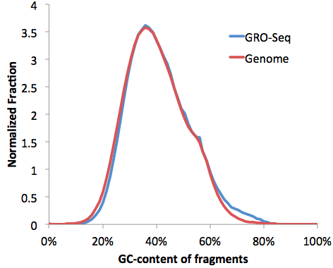
We can confirm the GC-distribution by opening the "tagGCcontent.txt" and "genomeGCcontent.txt" file in the IMR90-GroSeq directory and plotting together in EXCEL
It's also a good idea to check the nucleotide frequencies as a function of distance along the reads. Opening "tagFreqUniq.txt" and graphing with EXCEL:
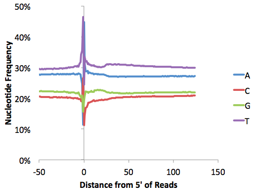
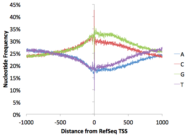
As with almost any sequencing technique, there are extreme nucleotide preferences at the 5' region where the reads at ligated to adapters. There is a little bit more G than C and T than A (normally G/C and A/T should track with one another), but this imbalance reflects levels of nucleotides downstream of the TSS minus the GC-enrichment and probably reflects natural nucleotide imbalance found in transcribed regions (graph below made with annotatePeaks.pl tss hg18 -size 2000 -hist 1 -di > output.txt)
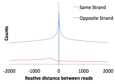
Also, examination of the autocorrelation data (open "tagAutocorrelation.txt" with EXCEL) yields a very typical GRO-Seq pattern. With any strand-specific RNA sequencing method, read are predominately on the same strand relative to one another. You'll notice a slight bump in the reads found on different strands - this is a manifestation of divergent transcription in the autocorrelation plot.
makeTagDirectory
IMR90-GroSeq/
-genome hg18 -checkGC GSM340901_lib1_aligned.bed
GSM340902_lib2_aligned.bed
This command will run out with something like this:
chucknorris@biowhat:~/tutorial$
makeTagDirectory GSM340901_lib1_aligned.bed
GSM340902_lib2_aligned.bed -genome hg18 -checkGC
Will parse file: GSM340901_lib1_aligned.bed
Will parse file: GSM340902_lib2_aligned.bed
Creating directory: IMR90-GroSeq and removing existing *.tags.tsv
Reading alignment file GSM340901_lib1_aligned.bed
Guessing that your alignment file is BED format
Reading alignment file GSM340902_lib2_aligned.bed
Guessing that your alignment file is BED format
Estimated genome size = 3078902552
Total Tags = 10751533.0
Total Positions = 9362481
Average tag length = 2.0
Median tags per position = 1
Average tags per position = 1.148364
Fragment Length Estimate: 33
Peak Width Estimate: 305
Autocorrelation quality control metrics:
Same strand fold enrichment: 1.6
Diff strand fold enrichment: 0.9
Same / Diff fold enrichment: 11.9
Guessing sample is strand specific RNA-Seq
Setting fragment length estimate to 75, edit tagInfo.txt to change
Checking GC bias...
Current Fragment length estimate: 75
Checking Tag/Fragment sequence for bias...
chr1
...
chrY
chrM
Avg Fragment GC% = 41.40%
Avg Expected GC% = 40.11%
Every time you get a new data set, there are a couple
things you want to keep your eye on. One is the average tags per
position, which describes how "clonal" the
experiment was. For RNA-Seq, you expect a higher
level of clonality, but with GRO-Seq, reads should be
found all over the genome and this value should be fairly
low (i.e. less than 2), unless you sequenced a ton of
reads. Another parameter to check for GRO-Seq is the
Same/Diff fold
enrichment, which should be high. If HOMER
doesn't guess the sample is strand specific RNA-Seq, there
may be problem with how the data was mapped or with how
the file is formatted. Finally, if the GC% distribution of
the fragments is extremely different from the
expected value (i.e. >10%), you might want to be very
careful proceeding.Will parse file: GSM340901_lib1_aligned.bed
Will parse file: GSM340902_lib2_aligned.bed
Creating directory: IMR90-GroSeq and removing existing *.tags.tsv
Reading alignment file GSM340901_lib1_aligned.bed
Guessing that your alignment file is BED format
Reading alignment file GSM340902_lib2_aligned.bed
Guessing that your alignment file is BED format
Estimated genome size = 3078902552
Total Tags = 10751533.0
Total Positions = 9362481
Average tag length = 2.0
Median tags per position = 1
Average tags per position = 1.148364
Fragment Length Estimate: 33
Peak Width Estimate: 305
Autocorrelation quality control metrics:
Same strand fold enrichment: 1.6
Diff strand fold enrichment: 0.9
Same / Diff fold enrichment: 11.9
Guessing sample is strand specific RNA-Seq
Setting fragment length estimate to 75, edit tagInfo.txt to change
Checking GC bias...
Current Fragment length estimate: 75
Checking Tag/Fragment sequence for bias...
chr1
...
chrY
chrM
Avg Fragment GC% = 41.40%
Avg Expected GC% = 40.11%
We can confirm the GC-distribution by opening the "tagGCcontent.txt" and "genomeGCcontent.txt" file in the IMR90-GroSeq directory and plotting together in EXCEL
It's also a good idea to check the nucleotide frequencies as a function of distance along the reads. Opening "tagFreqUniq.txt" and graphing with EXCEL:
As with almost any sequencing technique, there are extreme nucleotide preferences at the 5' region where the reads at ligated to adapters. There is a little bit more G than C and T than A (normally G/C and A/T should track with one another), but this imbalance reflects levels of nucleotides downstream of the TSS minus the GC-enrichment and probably reflects natural nucleotide imbalance found in transcribed regions (graph below made with annotatePeaks.pl tss hg18 -size 2000 -hist 1 -di > output.txt)
Also, examination of the autocorrelation data (open "tagAutocorrelation.txt" with EXCEL) yields a very typical GRO-Seq pattern. With any strand-specific RNA sequencing method, read are predominately on the same strand relative to one another. You'll notice a slight bump in the reads found on different strands - this is a manifestation of divergent transcription in the autocorrelation plot.
Creating UCSC Visualization Files
To visualize GRO-Seq
experiments in the UCSC Genome Browser, we'll run the makeUCSCfile command
(more info here). Since
GRO-Seq is strand specific, we need to specify options to
ensure it is visualized on separate strands. For our
example:
To make the resulting file only 50 MB (default), HOMER will randomly remove 60% of the data points (replaced with their average). You may want to try:
makeUCSCfile IMR90-GroSeq/ -o auto -strand
separate
To make the resulting file only 50 MB (default), HOMER will randomly remove 60% of the data points (replaced with their average). You may want to try:
- Changing "-fsize
<#>" to a very high number (i.e. 10e10)
so that it does not remove any points). However,
there is a greater chance UCSC will time out when
trying to upload the larger file, so you'll just have
to try it out and see what happens.
- Make two separate files using "-strand +" and "-strand -" (save them to different file names).
- Make a bigWig
file using the "-strand"
option (covered here).
The other parameter to play
around with is the fragment length ("-fragLengh <#>").
This will adjust how much coverage each tag generates in
the output.
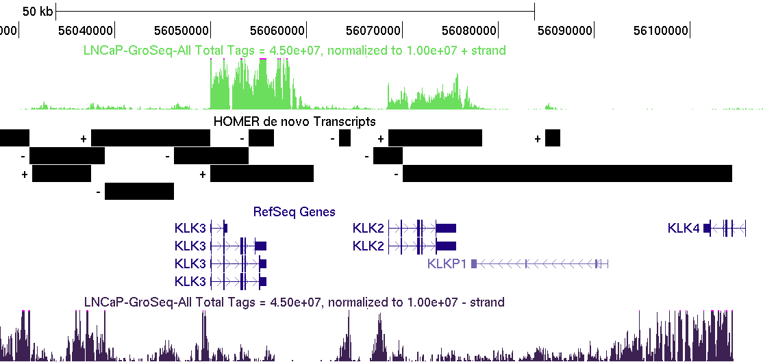
After you get the track you want, upload it to the UCSC Genome Browser. First step - select the hg18 version of the human genome. This is important - you always want to make sure you have the correct genome version!!! Then click on "add custom tracks", and upload the "IMR90-GroSeq.ucsc.bedGraph.gz" file in the "IMR90-GroSeq/" directory. Below is an example of the region at "chr14:73,956,837-74,768,357" (colors may differ since they are selected randomly)
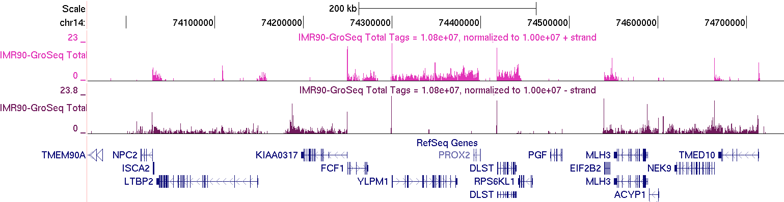
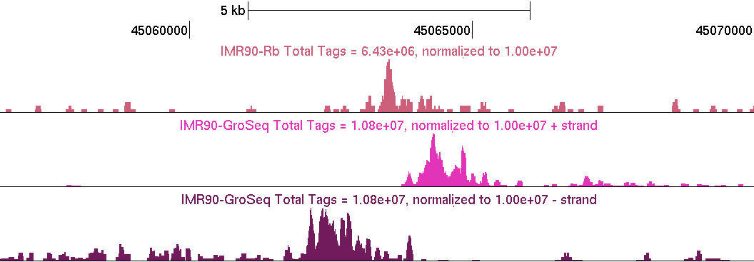
GRO-Seq data should "coat" annotated gene bodies as you see above. Usually there is a high number of reads right at the TSS where RNA polymerase II is frequently found "paused". There will also be places outside of gene bodies with GRO-Seq read coverage, such as near transcription factor binding sites. Below is an example of a distal pRb binding site (Not near a TSS, on chr12) with the typical GRO-Seq signature that is near transcription factor binding sites (pRb UCSC Track).
After you get the track you want, upload it to the UCSC Genome Browser. First step - select the hg18 version of the human genome. This is important - you always want to make sure you have the correct genome version!!! Then click on "add custom tracks", and upload the "IMR90-GroSeq.ucsc.bedGraph.gz" file in the "IMR90-GroSeq/" directory. Below is an example of the region at "chr14:73,956,837-74,768,357" (colors may differ since they are selected randomly)
GRO-Seq data should "coat" annotated gene bodies as you see above. Usually there is a high number of reads right at the TSS where RNA polymerase II is frequently found "paused". There will also be places outside of gene bodies with GRO-Seq read coverage, such as near transcription factor binding sites. Below is an example of a distal pRb binding site (Not near a TSS, on chr12) with the typical GRO-Seq signature that is near transcription factor binding sites (pRb UCSC Track).
Creating Histograms of GRO-Seq reads
GRO-Seq reads have a special
distribution near regions of transcription initiation
(e.g. near TSS). Transcription proceeds divergently
from the TSS in each direction. To create a
histogram of GRO-Seq reads near the TSS, use the annotatePeaks.pl
program in histogram mode (add "-hist <#>").
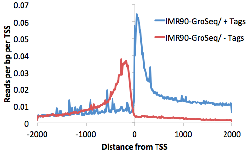
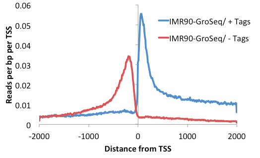
This will produce a histogram text file from -2000 to 2000 at 10 bp resolution (change with the "-hist <#>" parameter). Graphing the 3rd and 4th columns (that separate reads by strand) with EXCEL:
annotatePeaks.pl tss hg18 -size 4000 -hist 10
-d IMR90-GroSeq/ > outputFile.txt
This will produce a histogram text file from -2000 to 2000 at 10 bp resolution (change with the "-hist <#>" parameter). Graphing the 3rd and 4th columns (that separate reads by strand) with EXCEL:
One problem with GRO-Seq (or
any RNA-Seq) data is that there are some positions that
have a very high
density of reads, such as snoRNAs/rRNA
contamination. These sites will appear as "spikes"
in the histogram. To smooth this out, you can add
the option "-pc <#>"
(e.g. "-pc 3") to
limit the number or reads considered at each unique
position to # (or 3, in this example).
annotatePeaks.pl tss hg18 -size 4000 -hist 10
-d IMR90-GroSeq/ -pc 3 > outputFile.txt
Try the following (pRB peak file):
getDistalPeaks.pl rb.peaks.hg18.txt hg18 >
rb.distalPeaks.txt
annotatePeaks.pl rb.distalPeaks.txt hg18 -size 4000 -hist 25 -d IMR90-GroSeq -pc 1 > outputFile.txt
annotatePeaks.pl rb.distalPeaks.txt hg18 -size 4000 -hist 25 -d IMR90-GroSeq -pc 1 > outputFile.txt
This will make a histogram around the distal pRb peaks.
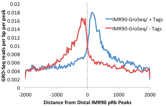
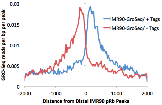
However, many of the peaks are found within introns, so the level of background is relatively high. getDistalPeaks.pl has additional options to isolate only intergenic peaks ("-intergenic").
getDistalPeaks.pl rb.peaks.hg18.txt hg18 -intergenic
> rb.distalPeaks.txt
annotatePeaks.pl rb.distalPeaks.txt hg18 -size 4000 -hist 25 -d IMR90-GroSeq -pc 1 > outputFile.txt (same as before)
annotatePeaks.pl rb.distalPeaks.txt hg18 -size 4000 -hist 25 -d IMR90-GroSeq -pc 1 > outputFile.txt (same as before)
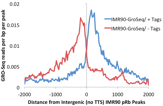
One more optimization for this process is to remove transcription factor peaks near the TTS where RNA polymerase often continues for several kB past the end of the gene. Removal of peaks from this region further reduce the background caused by read-through trancripts (add "-noTTS" option remove peaks within 10kb of the TTS).
getDistalPeaks.pl rb.peaks.hg18.txt hg18 -intergenic
-noTTS > rb.distalPeaks.txt
annotatePeaks.pl rb.distalPeaks.txt hg18 -size 4000 -hist 25 -d IMR90-GroSeq -pc 1 > outputFile.txt (same as before)
annotatePeaks.pl rb.distalPeaks.txt hg18 -size 4000 -hist 25 -d IMR90-GroSeq -pc 1 > outputFile.txt (same as before)
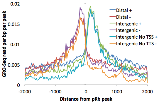
Placed on top of one another you can get a better sense for how the "upstream" read-through signal is smaller using more refined lists:
Analyzing GRO-Seq: de
novo transcript identification
To find transcripts directly
from GRO-Seq, use the findPeaks
command:
findPeaks <tag directory> -style groseq
-o auto
i.e. findPeaks Macrophage-GroSeq -style groseq -o auto
i.e. findPeaks Macrophage-GroSeq -style groseq -o auto
GRO-Seq analysis does not make use of an control tag directory
Basic Idea behind GRO-Seq Transcript identification
Finding transcripts using
strand-specific GRO-Seq data is not trivial.
GRO-Seq measures the production of nascent RNA, and is
capable of revealing the loction of protein coding
transcripts, promoter anti-sense transcripts, enhancer
templated transcripts, long and short functional
non-coding and miRNA transcripts, Pol III and Pol I
transcripts, and whatever else is being transcribed in
the cell nucleus. Identification and quantifiction
of these transcripts is important for downstream
analysis. Traditional RNA-Seq tools mainly focus
on mRNA, which has different features than GRO-Seq, and
are generally not useful for identifying GRO-Seq
transcripts.
Important NOTE: Just as with ChIP-Seq, not all GRO-Seq data was created equally. Data created by different labs can have features that make it difficult to have an single analysis technique that works perfectly for each one. As such, there are many parameters to play with the help get the desired results.
A large number of assumptions go into the analysis. In a nutshell, findPeaks tracks along each strand of each chromosome, searching for regions of continous GRO-Seq signal. Once it encounters high numbers of GRO-Seq reads, it starts a transcript. If the signal decreases significantly or disappears, the putative transcript is stopped. If the signal increases significantly (and sustainably), then a new transcript is considered from that point on. If the signal spikes, but overall does not increase over a large distance, it is considered an artifact or pause site and not considered in the analysis. Below is a chart that helps explain how the transcript detection works:
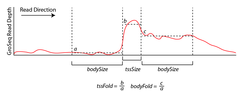
By default, new transcripts are created when the tssFold exceeds 4 and bodyFold exceed 3 ("-tssFold <#>", "-bodyFold <#>"). A small pseudo-count is added to the tag count from region a above to avoid dividing by zero and helps serve to set a minimum threshold for transcript detection ("-pseudoCount <#>", default: 1). Most transcripts show robust signal at the start of the transcript, and the tssFold helps select for these regions with high accuracy. The bodyFold is important for distinguishing between "spikes" in signal and real start sites; if a transcript is real, it's likely that increased levels of transcription follow behind the putative TSS. If the signal is roughly equal before and after the putative TSS, it is more likely to be an artifact.
To increase senstivity, HOMER tries to adjust the size of the bodySize parameter above since it essentially defines the resolution of the detected transcript. If there are a large number of GRO-Seq tags in a region, the bodySize can be small since there is adequate data to estimate the location of the transcript. However, if the data is relatively sparse, the bodySize needs to be large to get a reliable estimate of the level of the transcript. The minimum and maximum bodySizes are 600 and 10000 bp ("-minBodySize <#>", "-maxBodySize <#>"). HOMER uses the smallest bodySize that contains at least x number of tags, where x is determined as the number of tags where the chance of detecting a bodyFold change is less than 0.00001 assuming the read depth varies according to the poisson distribution (adjustable with "-confPvalue <#>", or directly with "-minReadDepth <#>"). The basic idea is that the threshold for tag counts must be high enough that we don't expect it to vary too much by chance.
Using uniquely mappable regions to improve results
Since some transcripts
cover very large regions, there are many places where
genomic repeats interrupt the GRO-Seq signal of
continous transcripts. To help deal with this
problem, HOMER can take advantage of mappability
information to help estimate transcript levels where
uniquely mapping sequencing reads is not possible.
In general this information is not really that helpful
for ChIP-Seq analysis, but in this case it can make an
important difference. For now, HOMER only take
specially formatted binary files available below.
To use them, download the appropriate version and unzip
the archive:
To use the uniq-map information, specify the location of the unzipped directory on the command line with "-uniqmap <directory>":
The uniqmap files above were generated assuming a 50nt read length. In reality, this will work reasonably well over a range of different nucleotide lengths.
Generating uniqmap files:
To use the uniq-map information, specify the location of the unzipped directory on the command line with "-uniqmap <directory>":
findPeak
Macrophage-GroSeq/ -style groseq -o auto -uniqmap
mm9-uniqmap/
The uniqmap files above were generated assuming a 50nt read length. In reality, this will work reasonably well over a range of different nucleotide lengths.
Generating uniqmap files:
Unfortunately, generating your own uniqmap files is a clunky procedure. However, you can do it by following these steps:
- Place the genome FASTA files for the genome of interest in a directory. There MUST be only one entry per file (i.e. chr1.fa, chr2.fa, chr3.fa). Unfortunately, the programs will not accept a single FASTA file will all of the chromosomes.
- Next, run the getMappableRegions command. This will eat up a ton of memory, which can be scaled by adjusting the first argument which sets the number of sequences that are analyzed in parallel. The program takes a while on mammalian genomes (~day). The second argument is the length of the reads you want to consider unique: "getMappableRegions 1000000000 50 *.fa > out.50nt.txt"
- Next run a utility program to create the uniqmap directory: "homerTools special uniqmap uniqmapDirectory/ out.50nt.txt". The "uniqmapDirectory/" can then be used with the findPeaks command.
GRO-Seq analysis output
Running findPeaks in
groseq mode will produce a file much like the one
produced for traditional peak finding, complete with a
header section listing the parameters and statistics
from the analysis. HOMER can also produce a GTF
(gene transfer format) file for use with various
programs. If "-o
auto" is used to specify output, a
"transcripts.gtf" file will be created in the tag
directory. Otherwise, you can specify the name of
the GTF output file by use "-gtf <filename>". The GTF
file can also be easily uploaded to the UCSC Genome
Browser to visualize your transcripts.
The GRO-Seq transcript
detection works pretty well, but is likely to get some
face-lifts in the near future.

Can't figure something out? Questions, comments, concerns, or other feedback:
cbenner@ucsd.edu