HOMER
Software for motif discovery and next-gen sequencing analysis
HOMER Motif Discovery Workflow
Regardless of how you invoke HOMER, the same basic steps are
executed to discover regulatory elements:Preprocessing:
1. Extraction of Sequences (findMotifs.pl/findMotifsGenome.pl)
If genomic regions are
provided as input, the appropriate genomic DNA is
extracted from the provided FASTA file or HOMER genome
annotation files. If gene accession numbers are
provided, the appropriate promoter regions are selected
from a table of promoter sequences.
2. Background Selection (findMotifs.pl/findMotifsGenome.pl)
If the background sequences
were not explicitly defined, HOMER will automatically
select them for you. If you are using genomic
positions, sequences will be randomly selected from the
genome, matched for GC% content (to make GC normalization
easier in the next step). HOMER2 now offers additional
control for how background sequences can be selected,
particularly in situations where you want to control for
positional sequence bias. If you are using promoter based
analysis, all promoters (except those chosen for analysis)
will be used as background. Custom background
regions can be specified with "-bg <file>".
3. GC Normalization (findMotifs.pl/findMotifsGenome.pl)
Sequences in the target and
background sets are then binned based on their GC-content
(5% intervals). Background sequences are weighted to
resemble the same GC-content distribution observed in the
target sequences. This helps avoid HOMER avoid
simply finding motifs that are GC-rich when analyzing
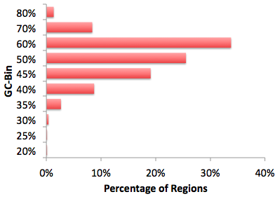
sequences from CpG Islands. To perform CpG%
normalization instead of GC%(G+C) normalization, use "-cpg". An
example of the GC%-distribution of regions from a ChIP-Seq
experiment:

4. Autonormalization (homer2/findMotifs.pl/findMotifsGenome.pl)
Often the target sequences
have an imbalance in the sequence content other than
GC%. This can be caused by biological phenomenon,
such as codon-bias in exons, or experimental bias caused
by preferential sequencing of A-rich stretches etc.
If these sources of bias are strong enough, HOMER will
lock on to them as features that significantly
differentiate the target and background sequences.
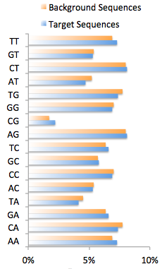
HOMER now offers autonormalization as a technique to
remove (or partially remove) imbalances in short oligo
sequences (i.e. AA) by assigning weights to background
sequences. The procedure attempts to minimize the
difference in short oligo frequency (summed over all
oligos) between target and background data sets. It
calculates the desired weights for each background
sequence to help minimize the error. Due to the
complexity of the problem, HOMER uses a simple
hill-climbing approach by making small adjustment in
background weight at a time. It also penalizes large
changes in background weight to avoid trivial solutions
that a increase or decrease the weights of outlier
sequences to extreme values. The length of short
oligos is controlled by the "-nlen <#>" option.

Discovering Motifs de
novo (homer2)
By default,
HOMER uses the new homer2 version of the program for
motif finding. If you wish to use the old
version when running any of the HOMER family of
programs, add "-homer1"
to the command line.
5. Parsing input sequences into an Oligo Table
Input sequences parsed in
to oligos of desired motif length, and read into an
Oligo Table. The Oligo Table hold each unique
oligo in the data set, remembering how many times it
occurs in the target and background sequences.
This is done to make searching for motif (which are
essentially collections of oligos) much more
efficient. However, this also destroys the
relationship between individual oligos and their
sequence of origin.
6. Oligo Autonormalization (optional)
While the
Autonormalization described in step 4 above is applied
to full sequences (i.e. ~200 bp), you can also apply the
autonormalization concept to the Oligo Table. The
idea is still to equalize the smaller oligo lengths
(i.e. 1,2,3 bp) within the longer oligos (i.e. 10,12,14
bp etc.). This is a little more dangerous since
the total number of motif-length oligos can be very
large (i.e. 500k for 10 bp, much more for longer
motifs), meaning there are a lot of weights to
"adjust". However, this can help if there is an
extreme sequence bias that you might be having trouble
scrubbing out of the data set (the "-olen <#>"
option).
7. Global Search phase
After creating (and
possibly normalizing) the Oligo Table, HOMER conducts a
global search for enriched "oligos". The basic
idea is that if a "Motif" is going to be enriched, then
the oligos considered part of the motif should also be
enriched. First, HOMER screens each possible oligo
for enrichment. To increase sensitivity, HOMER
then allows mismatches in the oligo when searching for
enrichment. To speed up this process, which can be
very resource consuming for longer oligos with a large
number of possible mismatches, HOMER will skip oligos
when allowing multiple mismatches if they were not
promising, for example if they had more background
instances than target instances, or if allowing more
mismatches results in a lower enrichment value.
The "-mis <#>"
controls how many mismatches will be allowed.
Calculating Motif Enrichment:
Calculating Motif Enrichment:
Motif enrichment is
calculated using either the cumulative hypergeometric
or cumulative binomial distributions. These two
statistics assume that the classification of input
sequences (i.e. target vs. background) is independent
of the occurrence of motifs within them. The
statistics consider the total number of target
sequences, background sequences and how many of each
type contains the motif that is being checked for
enrichment. From these numbers we can calculate
the probability of observing the given number (or
more) of target sequences with the motif by chance if
we assume there is no relationship between the target
sequences and the motif. The hypergeometric and
binomial distributions are similar, except that the
hypergeometric assumes sampling without replacement,
while the binomial assumes sampling with
replacement. The motif enrichment problem is
more accurately described by the hypergeometric,
however, the binomial has advantages. The
difference between them is usually minor if there are
a large number of sequences and the background
sequences >> target sequences. In these
cases, the binomial is preferred since it is faster to
calculate. As a result it is the default
statistic for findMotifsGenome.pl
where the number of sequences is typically
higher. However, if you use your own background
that has a limited number of sequences, it might be a
good idea to switch to the hypergeometric (use "-h" to force use
of the hypergeometric). findMotifs.pl
expects a smaller number for promoter analysis and
uses the hypergeometric by default.
One important note: Since HOMER uses an Oligo Table for much of the internal calculations of motif enrichment, where it does not explicitly know how many of the original sequences contain the motif, it approximates this number using the total number of observed motif occurrences in background and target sequences. It assumes the occurrences were equally distributed among the target or background sequences with replacement, were some of the sequences are likely to have more than one occurrence. It uses the expected number sequences to calculate the enrichment statistic (the final output reflects the actual enrichment based on the original sequences).
One important note: Since HOMER uses an Oligo Table for much of the internal calculations of motif enrichment, where it does not explicitly know how many of the original sequences contain the motif, it approximates this number using the total number of observed motif occurrences in background and target sequences. It assumes the occurrences were equally distributed among the target or background sequences with replacement, were some of the sequences are likely to have more than one occurrence. It uses the expected number sequences to calculate the enrichment statistic (the final output reflects the actual enrichment based on the original sequences).
8. Matrix Optimization
HOMER takes the most
enriched oligos from the global optimization step,
transforms them into simple position specific
probability matrices, and further optimizes them with a
sensitive local optimization algorithm. This step
is performed separately for each oligo, and will create
the "motif probability matrix" as well as determine the
optimal detection threshold to maximize the enrichment
of the motif in the target vs. background
sequences. The detection threshold is simply done
by scoring each oligo in the data to the probability
matrix, and then sorting the oligos by their similarity
to the matrix. HOMER then steps down the list,
effectively decreasing the detection threshold,
including more and more oligos until an optimal
enrichment is found. After this step, HOMER will
create several new probability matrices based on the
oligos found in different detection thresholds and check
which one has the highest enrichment. This process
is repeated until the enrichment can no longer be
improved, producing a final motif.
9. Mask and Repeat
After the first "promising
oligo" is optimized into a motif, the sequences bound by
the motif to are removed from the analysis and the next
promising oligo is optimized for the 2nd motif, and so
on. This is repeated until the desired number of
motifs are found ("-S
<#>", default: 25). This is where
the there is an important difference between the old
(homer) and new (homer2) versions. The old version
of homer would simply mask the oligos bound by the motif
from the Oligo Table. For example if the motif was
GAGGAW then GAGGAA and GAGGAT would be removed from the
Oligo Table to avoid having the next motif find the same
sequences. However, if GAGGAW was enriched in the
data, there is a good chance that any 6-mer oligo like
nGAGGA or AGGAWn would also be somewhat enriched in the
data. This would cause homer to find multiple
versions of the same motif and provide a little bit of
confusion in the results.
To avoid this problem in the new version of HOMER (homer2), once a motif is optimized, HOMER revisits the original sequences and masks out the oligos making up the instance of the motif as well as well as oligos immediately adjacent to the site that overlap with at least one nucleotide. This helps provide much cleaner results, and allows greater sensitivity when co-enriched motifs. To make revert back to the old way of motif masking with homer2, specify "-quickMask" at the command line. You can also run the old version with "-homer1".
To avoid this problem in the new version of HOMER (homer2), once a motif is optimized, HOMER revisits the original sequences and masks out the oligos making up the instance of the motif as well as well as oligos immediately adjacent to the site that overlap with at least one nucleotide. This helps provide much cleaner results, and allows greater sensitivity when co-enriched motifs. To make revert back to the old way of motif masking with homer2, specify "-quickMask" at the command line. You can also run the old version with "-homer1".
Screening for Enrichment of Known Motifs (homer2):
10. Load Motif Library
In order to search for
Known Motifs in your data, HOMER loads a list of
previously determined motifs from previous data.
You can also add you own motifs by specifying them at
the command line ("-mknown
<file>") or by editing the primary file
("data/knownTFs/known.motifs"). HOMER doesn't
screen all of TRANSFAC - partially due to motif quality
(which can be low), and paritically due to the fact that
we need a detection threshold.
11. Screen Each Motif
To find the enrichment for
each motif, HOMER scans each sequence for instances of
the motif and calculates the final enrichment by
considering how many target vs. background sequences are
considered "bound". ZOOPS (zero or one occurence
per sequence) counting is used and the hypergeometric or
binomial is used to calculate the significance.
Motif Analysis Output:
12. Motif Files (homer2, findMotifs.pl,
findMotifsGenome.pl)
The true output of HOMER
are "*.motif" files which contain the information
necessary to identify future instance of motifs.
They are reported in the output directories from
findMotifs.pl and findMotifsGenome.pl. A typical
motif file will look something like:
>ASTTCCTCTT 1-ASTTCCTCTT 8.059752 -23791.535714 0 T:17311.0(44 ...
0.726 0.002 0.170 0.103
0.002 0.494 0.354 0.151
0.016 0.017 0.014 0.954
0.005 0.006 0.027 0.963
0.002 0.995 0.002 0.002
0.002 0.989 0.008 0.002
0.004 0.311 0.148 0.538
0.002 0.757 0.233 0.009
0.276 0.153 0.030 0.542
0.189 0.214 0.055 0.543
The first row starts with a ">" followed by various information, and the other rows are the positions specific probabilities for each nucleotide (A/C/G/T). The header row is actually TAB delimited, and contains the following information:
- ">" + Consensus sequence (not actually used for anything, can be blank) example: >ASTTCCTCTT
- Motif name (should be unique if several motifs are in the same file) example: 1-ASTTCCTCTT or NFkB
- Log odds detection threshold, used to determine bound vs. unbound sites (mandatory) example: 8.059752
- log P-value of enrichment, example: -23791.535714
- 0 (A place holder for backward compatibility, used to describe "gapped" motifs in old version, turns out it wasn't very useful :)
- Occurence Information separated by commas, example: T:17311.0(44.36%),B:2181.5(5.80%),P:1e-10317
- T:#(%) - number of target sequences with motif,
% of total of total targets
- B:#(%) - number of background sequences with motif, % of total background
- P:# - final enrichment p-value
- Motif statistics separated by commas, example: Tpos:100.7,Tstd:32.6,Bpos:100.1,Bstd:64.6,StrandBias:0.0,Multiplicity:1.13
- Tpos: average position of motif in target sequences (0 = start of sequences)
- Tstd: standard deviation of position in target sequences
- Bpos: average position of motif in background sequences (0 = start of sequences)
- Bstd: standard deviation of position in background sequences
- StrandBias: log ratio of + strand occurrences to - strand occurrences.
- Multiplicity: The averge number of occurrences
per sequence in sequences with 1 or more binding
site.
13. De novo motif output (findMotifs.pl/findMotifsGenome.pl/compareMotifs.pl)
HOMER takes the motifs
identified from de
novo motif discovery step and tries to process
and present them in a useful manner. An HTML page
is created in the output directory named
homerResults.html along with a directory named
"homerResults/" that contains all of the image and other
support files to create the page. These pages are
explicitly created by running a subprogram called "compareMotifs.pl".
Comparison of Motif Matrices:
Motifs are first checked for redundancy to avoid presenting the same motifs over and over again. This is done by aligning each pair of motifs at each position (and their reverse opposites) and scoring their similarity to determine their best alignment. Starting with HOMER v3.3, matrices are compared using Pearson's correlation coefficient by converting each matrix into a vector of values. Neutral frequencies (0.25) are used in where the motif matrices do not overlap.
The old comparison was done by comparing the probability matrices using the formula below which manages the expectations of the calulations by scrambling the nuclotide identities as a control. (freq1 and freq2 are the matrices for motif1 and motif2)
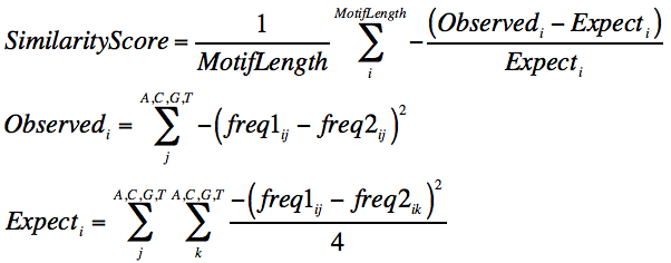
The output will be a score ranging from some lower bound (depending on the matrix frequencies) to 1, where 1 is complete similarity. By default the threshold for assigning similar motifs is 0.6, which is a reasonable cutoff in practice. This can be changed if you run compareMotifs.pl and change the "-reduceThresh <#>" parameter.
Comparison of Motif Matrices:
Motifs are first checked for redundancy to avoid presenting the same motifs over and over again. This is done by aligning each pair of motifs at each position (and their reverse opposites) and scoring their similarity to determine their best alignment. Starting with HOMER v3.3, matrices are compared using Pearson's correlation coefficient by converting each matrix into a vector of values. Neutral frequencies (0.25) are used in where the motif matrices do not overlap.
The old comparison was done by comparing the probability matrices using the formula below which manages the expectations of the calulations by scrambling the nuclotide identities as a control. (freq1 and freq2 are the matrices for motif1 and motif2)

The output will be a score ranging from some lower bound (depending on the matrix frequencies) to 1, where 1 is complete similarity. By default the threshold for assigning similar motifs is 0.6, which is a reasonable cutoff in practice. This can be changed if you run compareMotifs.pl and change the "-reduceThresh <#>" parameter.
Motifs are next compared
against a library of known motifs. For this step,
all motifs in JASPAR and the "known" motifs are used for
comparison. You can specify a custom motif library
using "-mcheck
<motif library file>" when using findMotifs[Genome].pl
or "-known <motif
library file>" when calling compareMotifs.pl
directly.
By default, it looks for the file "/path-to-homer/data/knownTFs/all.motifs" to find the motif to compare with the de novo motifs. If "-rna" is specified, it will load the file "/path-to-homer/data/knownTFs/all.rna.motifs".
An example of the output HTML is show below:
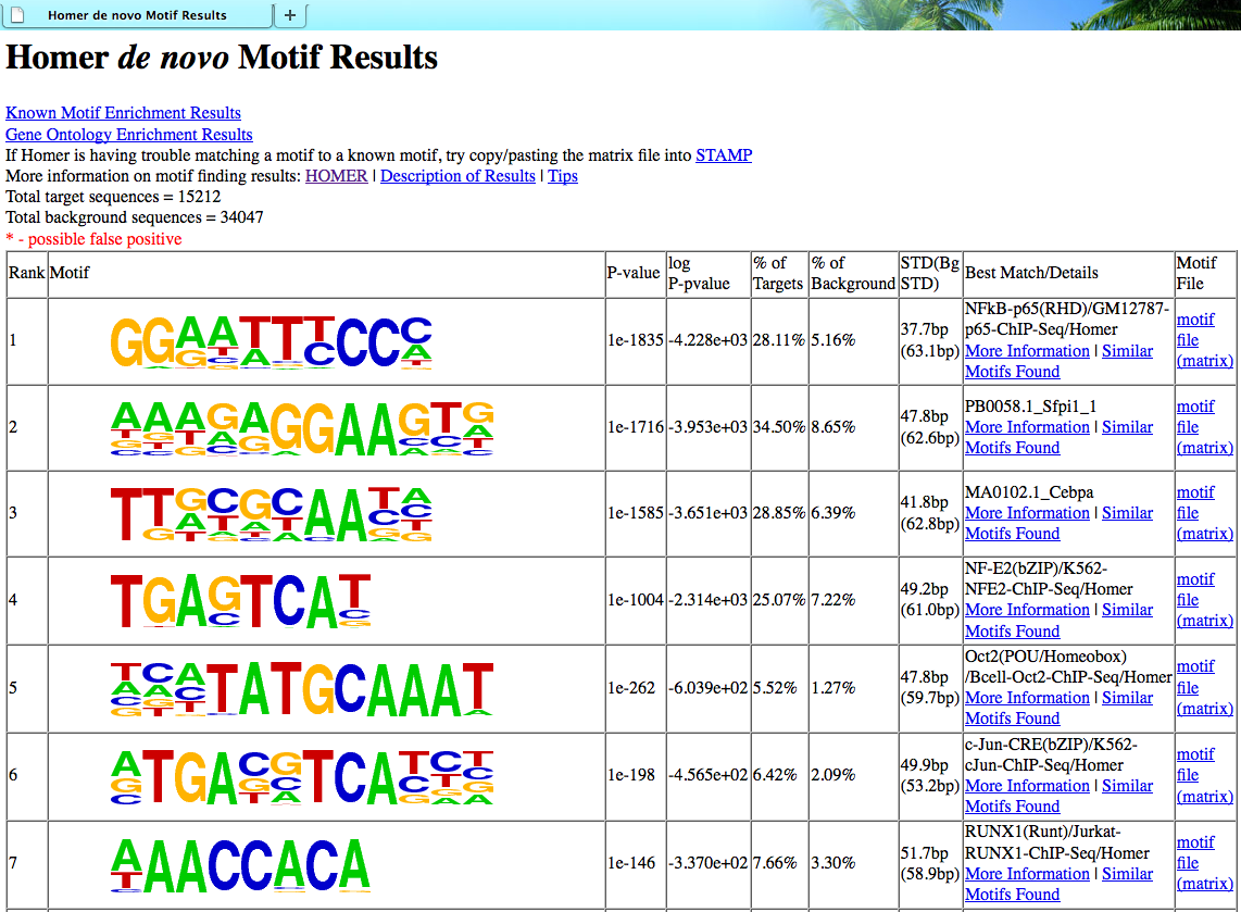
Depending on how the findMotifs[Genome].pl program that was executed, the "Known Motif Enrichment Results" and "Gene Ontology Enrichment Results" may or may not link to anything. Motifs are sorted based on p-value, and basic statistics about the motif (present in the motif files) is displayed.
The final column contains a link to the "motif file", which is important if you want to search for the motif in other sequences.
In the Best Match/Details column, HOMER will display the known motif which most closely matched with the de novo motif. It is very important that you TAKE THIS ASSIGNMENT WITH A GRAIN OF SALT!!!!! Unfortunately, sometimes the best match still isn't any good. Also, it is common that the "known" motif isn't any good to begin with. To investigate the assignment further, click on the "More Information" link which provides a page that looks like this:
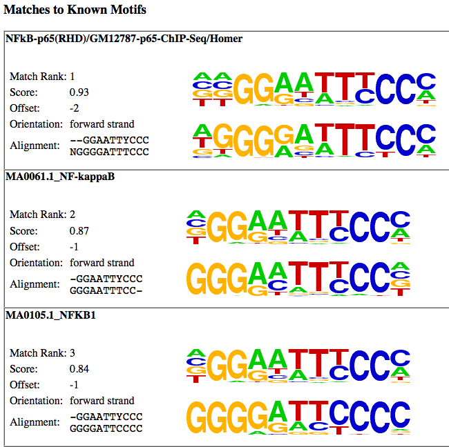
Followed by matches to known motifs. This section shows the alignments between the de novo motif and known motifs. It's important to check and see if these alignments look reasonable:
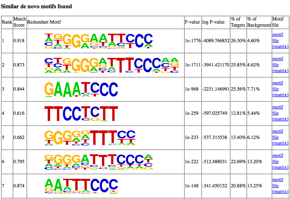
Clicking on the "similar motifs" will show the other de
novo motifs found during motif finding that resemble the
motif but had a lower enrichment value. It
contains a similar "header" as the "More Information"
link, but below it shows the motifs that were considered
similar. It is usually a good idea to check this
list over - sometimes a distinct motif will be grouped
incorrectly in the list because it shares a couple
residues.
To rerun this part of the analysis on any arbitrary set of motifs, simply run the "compareMotifs.pl" command (use without any command line parameters to get the usage options).
By default, it looks for the file "/path-to-homer/data/knownTFs/all.motifs" to find the motif to compare with the de novo motifs. If "-rna" is specified, it will load the file "/path-to-homer/data/knownTFs/all.rna.motifs".
An example of the output HTML is show below:

Depending on how the findMotifs[Genome].pl program that was executed, the "Known Motif Enrichment Results" and "Gene Ontology Enrichment Results" may or may not link to anything. Motifs are sorted based on p-value, and basic statistics about the motif (present in the motif files) is displayed.
The final column contains a link to the "motif file", which is important if you want to search for the motif in other sequences.
In the Best Match/Details column, HOMER will display the known motif which most closely matched with the de novo motif. It is very important that you TAKE THIS ASSIGNMENT WITH A GRAIN OF SALT!!!!! Unfortunately, sometimes the best match still isn't any good. Also, it is common that the "known" motif isn't any good to begin with. To investigate the assignment further, click on the "More Information" link which provides a page that looks like this:
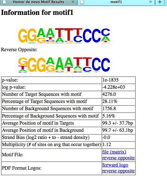
Basic Information:
The section contains basic information, including
links to the motif file (normal and reverse opposite)
and the pdf version of the motif logo.

Followed by matches to known motifs. This section shows the alignments between the de novo motif and known motifs. It's important to check and see if these alignments look reasonable:


To rerun this part of the analysis on any arbitrary set of motifs, simply run the "compareMotifs.pl" command (use without any command line parameters to get the usage options).
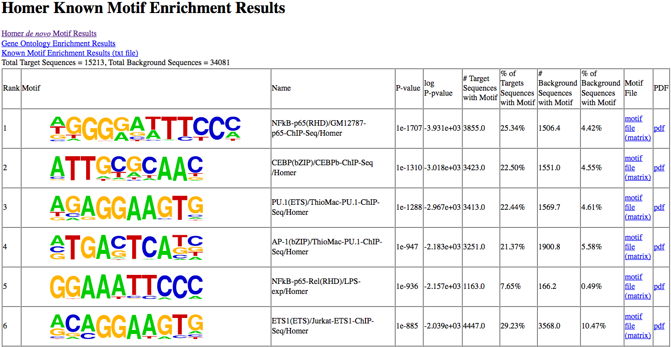
14. Known motif output
Known motif enrichment is
displayed as a HTML file (knownResults.html). The
page sorts the results based on enrichment and displays
basic information:


Can't figure something out? Questions, comments, concerns, or other feedback:
cbenner@ucsd.edu