
HOMER
Software for motif discovery and next-gen sequencing analysis
Creating and Normalizing Hi-C interaction/contact
Matrices
The most basic way to represent Hi-C data is in matrix
format, where the number of interactions can be reported
between sets of regions. Since it's difficult to
extract this data from the raw mapped reads, HOMER
provides tools create matrices from tag directories.
Most Hi-C tasks in HOMER revolve around the analyzeHiC
command. Below is a description of how to use it to
create matrices. analyzeHiC requires a Hi-C
tag directory (direction on creating one from FASTQ or
Alignment files can be found here). Newer versions of
HOMER strive to perform normalization of matrices on the
fly to accommodate different parameters for analysis.
Matrices that are normalized for interaction distance will
still trigger the creation of a HOMER-background model
though.
It is also worth noting that there are many other useful
ways to visualize Hi-C data. One highly recommended
way to visualize and 'surf' Hi-C data is to use Juicebox.
This requires generating a *.hic file from the experiment,
which is covered here.
Quick Reference:
analyzeHiC HicExp1TagDir/ -pos chr2:10,000,000-12,000,000 -res 3000 -window 15000 -balance > output.txt
#visualize "output.txt" with Treeview 3 or other heatmap/cluster visualization software
#resolution controls the sampling resolution, window controls the binning resolution (i.e. above it will pool reads in 15kb bins at 3kb intervals, i.e. overlapping intervals)
Quick Note about Hi-C Analysis
Hi-C is an unbiased assay of chromatin conformation, resulting in even read coverage across the entire genome. This, coupled with the fact that most Hi-C reads describe interactions at close linear distance along the chromosomes, results in relatively sparse read coverage for interactions between individual restriction fragments separated by great distance. This makes it difficult to find high-resolution interactions across long distances. To help describe how distal and/or inter-chromosomal regions co-localize, two general approaches are utilized:
- Increase the size of the regions [i.e. decrease the resolution] to boost the number of Hi-C reads used for interaction analysis. This is the most common and simplest technique used by most approaches (including HOMER). It's much easier to identify significant inter-chromosomal interactions between regions that are 100kb in size than regions that are only 5kb in size (essentially 20x more Hi-C reads to work with).
- Compare the profile of interactions regions participate in when comparing regions. The best example of this is calculating the correlation coefficient of the interaction profiles between two regions. The idea is that if two regions share interactions with several other regions, they are probably similar themselves (even if they do not have direct interaction evidence between them). This forms the basis of the PCA analysis, and uses the transitive property to link regions. If A interacts with C and D, and B interactions with C and D, perhaps A and B interact as well.
Running analyzeHiC
Changing the Resolution and Window Size of Analysis
HOMER uses two (related) notions of resolution. The first, "-res <#>" represents how frequent the genome is divided up into regions to analyze (i.e. the step-size of the analysis). The second, the window resolution "-window <#>", represents how large the region is expanded when counting reads. Usually the "-res <#>" should be smaller than the "-window <#>" - this will effectively analyze the data in overlapping window, which is useful for removing edge effects. For example a res of 50000 and a window of 100000 would mean that HOMER will analyze the regions 0-50k, 50k-100k, 100k-150k etc., but at each region it will look at reads from a region the size of 100k, so it would look at reads from -25k-75k, 25k-125k, 75k-175k, etc. This means HOMER will analyze data with overlapping windows. The principle advantage to this strategy is that you don't penalize features that span boundaries. For example:
analyzeHiC ES-HiC -pos chr1:10,000,000-13,000,000 -res 10000 -window 20000 > output.10kby20kResolution.txtKeep in mind that the resolution will also dictate the size of the output matrix. The command will warn you if your parameters seem unreasonable...
Specifying specific regions to analyze
-start <#> : starting position for analysis
-end <#> : end position for analysis
-pos <chr:start-end> : UCSC browser formatted position - if you're lazy like me, takes place of the -chr/-start/-end
If you only "-chr chr1" and do not specify a start and end, HOMER will simply visualize all of chr1. Regions will be created starting at position 0 to 1*resolution, then from 1*resolution to 2*resolution, etc. (i.e. 0-10kb, 10kb-20kb, 20kb-30kb) If an alternative start is specified, then regions will be created at start+0*resolution to start+1*resolution, start+1*resolution to start+2*resolution, etc (i.e. 205kb-215kb,215kb-225kb,...).
HOMER will normally make a symmetric matrix by default. If you want to specifically look at a matrix between two different regions:
-start2 <#> : starting position for analysis
-end2 <#> : end position for analysis
-pos2 <chr:start-end> : UCSC browser formatted position - if you're lazy like me, takes place of the -chr2/-start2/-end2
-vsGenome : compare to the rest of the genome
NOTE: Don't use -chr2/-start2/-end2/-pos2/-vsGenome unless you specified something with -chr/-start/-end/-pos etc. first.
Using these regions, HOMER will divide them into #-bp regions, where # is the resolution. HOMER doesn't allow you to cherry-pick several regions from different chromosomes. At least not using the -chr, -start, -end, and -pos options. (You could do this with peaks and the -p option).
You can arbitrarily define the regions you want to examine by providing a peak/BED file of the regions. However, these options work a little differently. In the case above (with -chr/-start/-end/-pos), HOMER will chop up the region into resolution sized chunks and perform the analysis. I.e. you provide a locus you want a detailed picture of. When providing a peak file, HOMER will only consider the center of the peak file and the surrounding "resolution-sized" region. It will not chop-up your peaks into resolution-sized chunks (unless you specify the "-chopify" option). In general, the "-p" option is more useful for looking at all CTCF peaks, for example, to see which are interacting. You can provide a peak/BED that effectively tiles a region, in which case it would mimic how -chr/-start/-end/-pos works, but give you the flexibility to define any region(s) you wanted. To specify a peak file containing regions to analyze with analyzeHiC:
-p2 <peak/BED file> : A second peak/BED file for non-symetrical matricies.
Keep in mind that an interaction matrix is probably only useful at 2000 x 2000 points - much bigger you can't really visualize it easily anymore (The file will also get really big...)
Matching the resolution of Peak/BED Files and
Resolution of analyzeHiC
The resulting file will contain only peaks at least 50000 bp from one another. Use this resulting file with analyzeHiC.
Visualizing the Interaction Matrix
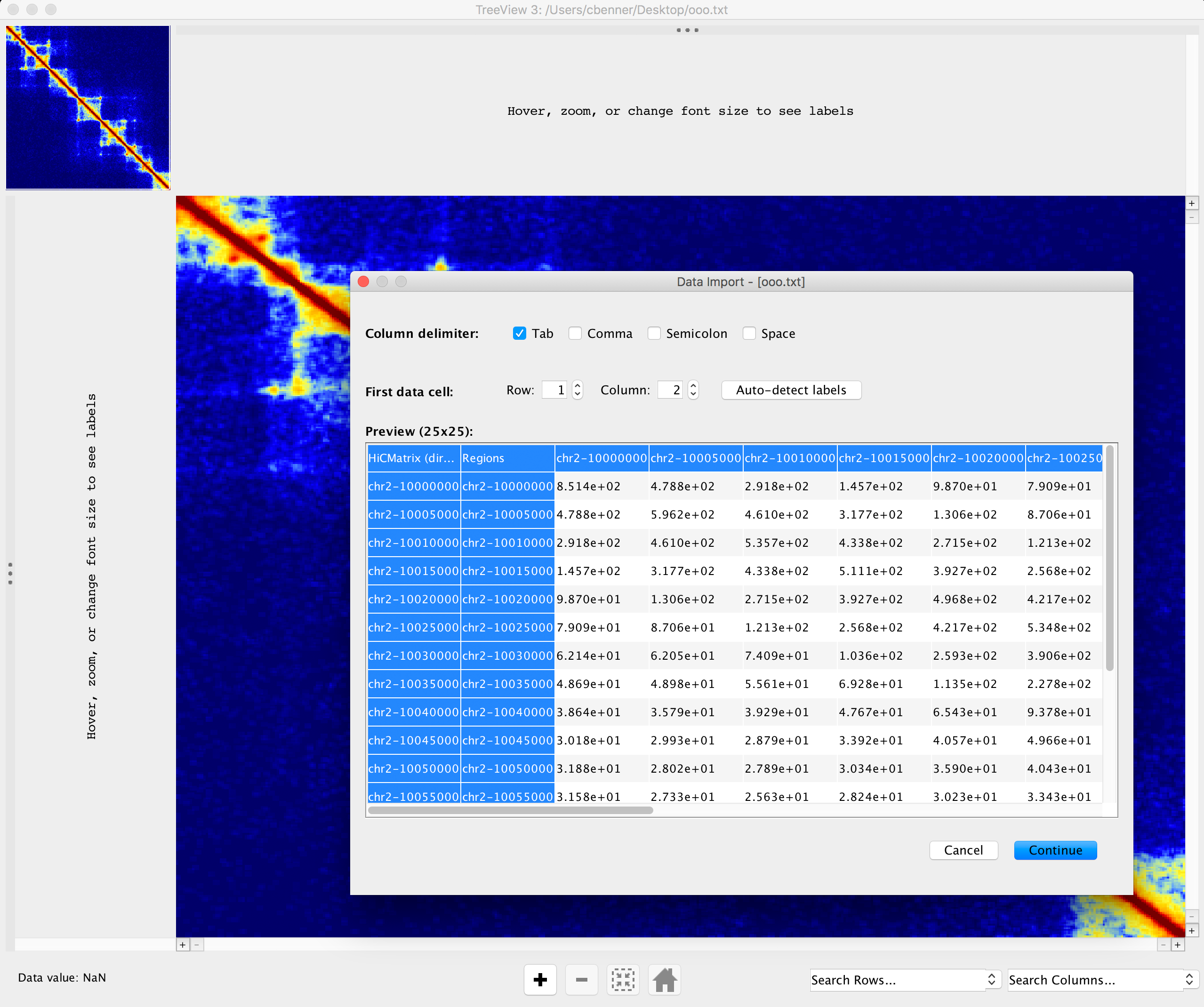
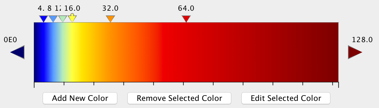
Analyze Hi-C will output a tab-delimited text file that can be used by other programs to generate a 'heatmap' or similar image. For interactive visualization, we recommend using Treeview 3 or other heatmap/cluster visualization software. The advantage of Treeview 3 over some other options is that it allows you to specify your own color scheme. For example, we like the following color scheme for ihskb normalization (which is used in most of the examples of Hi-C contact matrices below). The color scheme is linked to the filename, so you can temporarily name your files the same name to open them with Treeview 3 and have it automatically load the same color scheme:
Using a heatmap viewer like Treeview is great when viewing interactively as it allows you to modify the color scheme or zoom in on features, etc. However, if creating several matrices, we highly recommend using R or a python script (i.e. matplotlib) to generate them in batch.
Different types of normalization and analysis options
for Hi-C matrices
Output Information Options (choose only one ):
-coverageNorm (default)
-distNorm
-corr
Matrix Balancing
Using "-balance" will iteratively balance matrices to ensure the total interactions are the same for each region (i.e. row/column). This helps remove artifacts caused from differential Hi-C read coverage. However, regions with limited/low read coverage will have "inflated" interaction counts - so be careful trying to interpreting interactions from these regions.
Creating Relative Matrices
You can create a matrix which only analyzes contacts near the diagonal up to a maximum distance using the options "-relative" and "-maxDist <#>". This allows you to create a 'matrix' that excludes the relatively sparse interactions found between distal regions.
Other options:
-cpu <#> : (default: 1) Use multiple threads when performing analysis (only useful for in this case for the processing of multiple chromosomes or when creating a background model for -distNorm)
-std <#> : (default: 8) exclude the analysis of regions where the number of mapped reads exceeds the average number by 8 standard deviations (i.e. z-score greater than 8).
-min <#> : (default: 0.05) exclude the analysis of regions where the number of mapped reads is lower than this fraction of the average (default excludes regions with less than 5%)
-override : By default, HOMER will bail if you try to make a matrix that is too big. This option will remove the check and go ahead and make it anyway...
-log, -nolog : Will force the output of log (or linear) transformed values
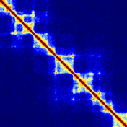
Examples of Hi-C matrices created with analyzeHiC
The following examples show how changing the -res and -window parameters can change how the contact matrix looks. Importantly, note that the default normalization (-ihskb) will automatically adjust the normalization so that the matrices are comparable across different parameters.
Consider the same 2.2 Mb region visualized with a resolution of 10kb or 25kb:
Now lets reduce the value resolution in half while keeping the window the same size to smooth out edge effects:analyzeHiC MDM-HiC/ -pos chr2:10000000-12200000 -res 10000 -window 10000 -balance > output.res10k.win10k.txt
analyzeHiC MDM-HiC/ -pos chr2:10000000-12200000 -res 25000 -window 25000 -balance > output.res25k.win25k.txt

analyzeHiC MDM-HiC/ -pos chr2:10000000-12200000 -res 5000 -window 10000 -balance > output.res5k.win10k.txt
analyzeHiC MDM-HiC/ -pos chr2:10000000-12200000 -res 12500 -window 25000 -balance > output.res12.5k.win25k.txt

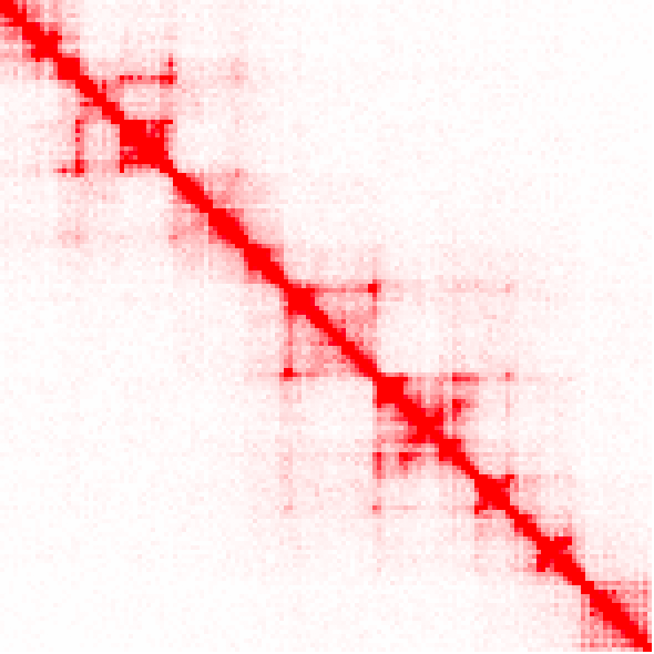
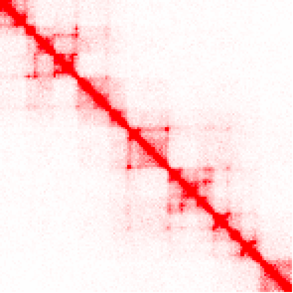
Example of raw counts, and the difference between unbalanced and balanced versions (keep in mind the interaction counts are very different than the ihskb normalization so they have been visualized in the 'standard red'):
analyzeHiC MDM-HiC/ -pos chr2:10000000-12200000 -res 15000 > output.raw.res15k.txt
analyzeHiC MDM-HiC/ -pos chr2:10000000-12200000 -res 15000 -balance > output.raw.res15k.balance.txt
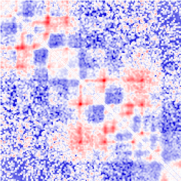
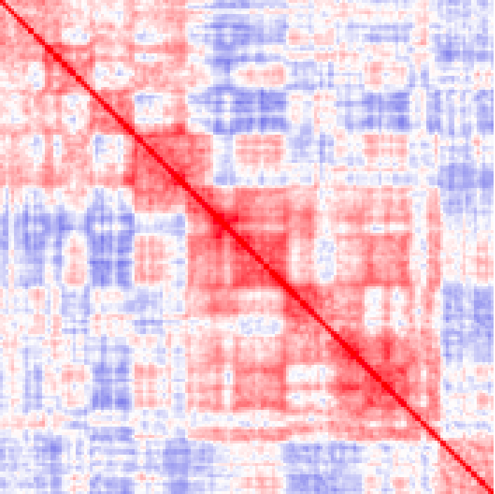
Example of distance normalized matrix (visualized as log2 ratios from -4 [blue] to +4 [red]) and a correlation matrix (-1 to 1):
analyzeHiC MDM-HiC/ -pos chr2:10000000-12200000 -res 15000 > output.raw.res15k.txt
analyzeHiC MDM-HiC/ -pos chr2:10000000-12200000 -res 15000 -balance > output.raw.res15k.balance.txt
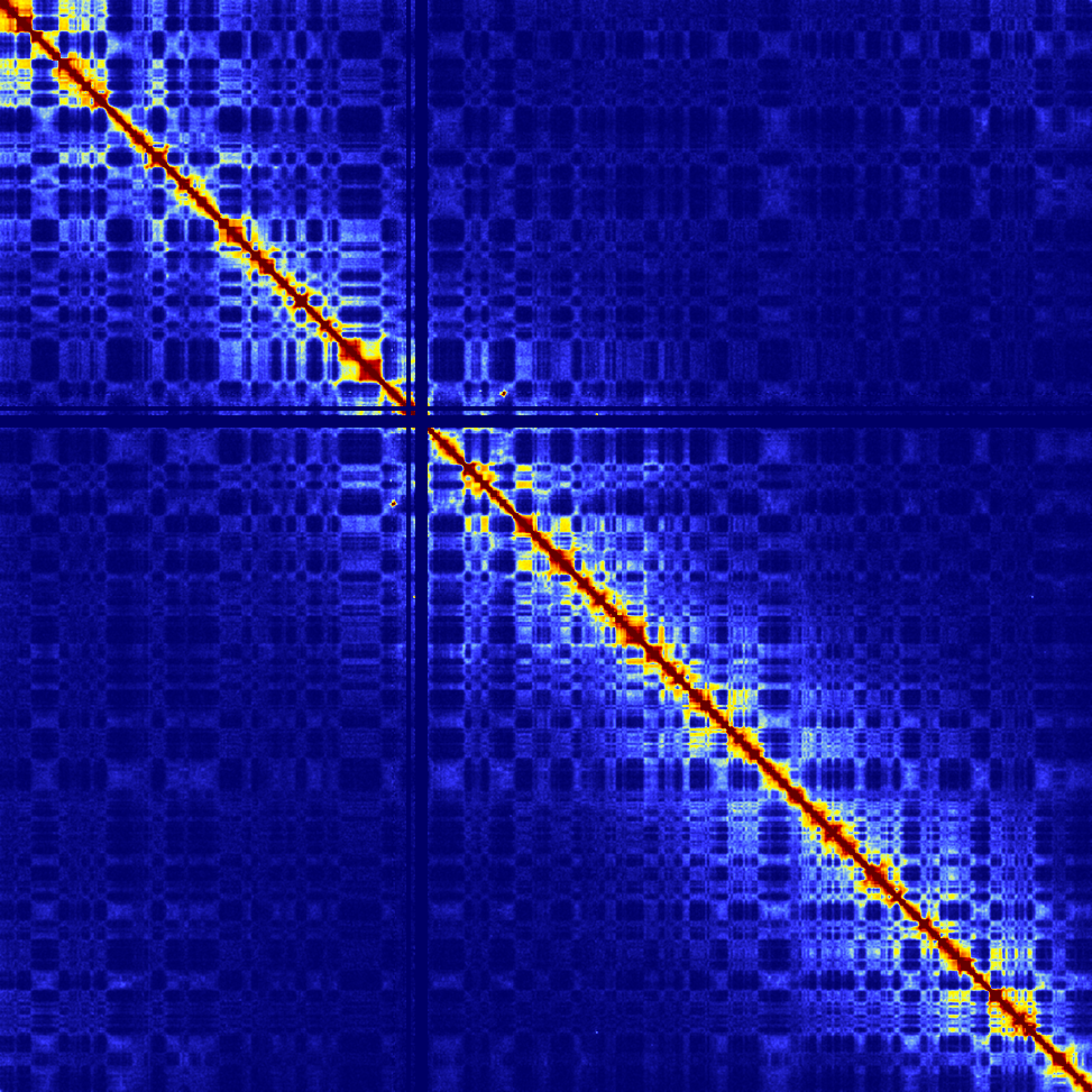
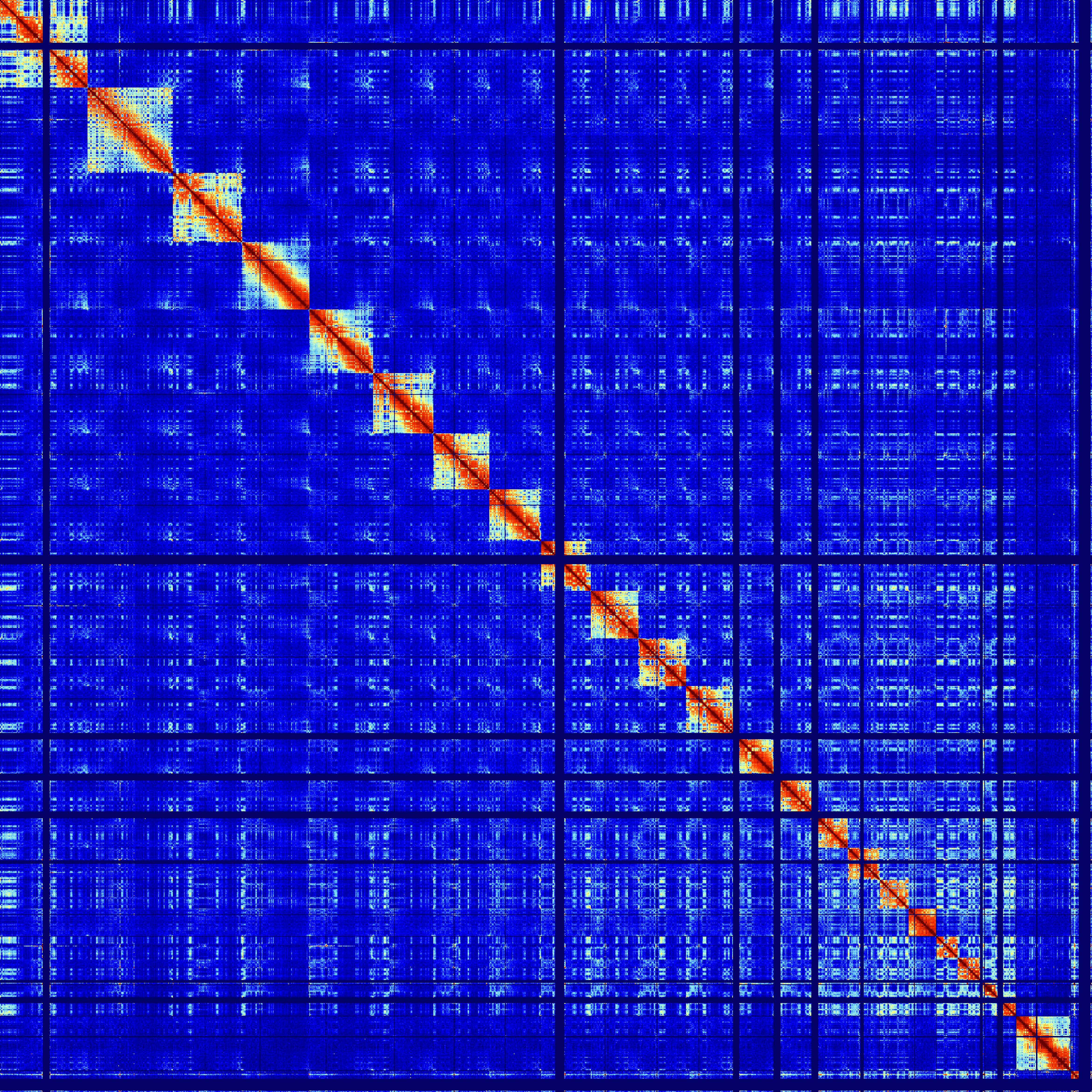
Example of visualizing an entire chromosome at 250kb resolution. Notice the characteristic checkerboard pattern that emerges as a result of chromatin compartments (note that the colors were adjusted from the original scheme such that they represent 1/100th of the original interaction density):
analyzeHiC MDM-HiC/ -chr chr2 -res 250000 -window 500000 -balance > output.chr2.250kres.txt
Example of visualizing the whole genome at 2 Mb resolution (colors are now 1/2000th the original color scheme):
analyzeHiC MDM-HiC/ -res 2000000 -balance > output.genome.2Mres.txt

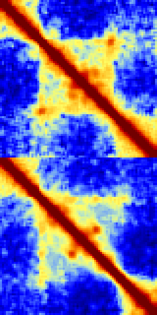
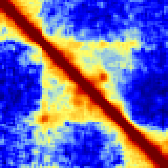
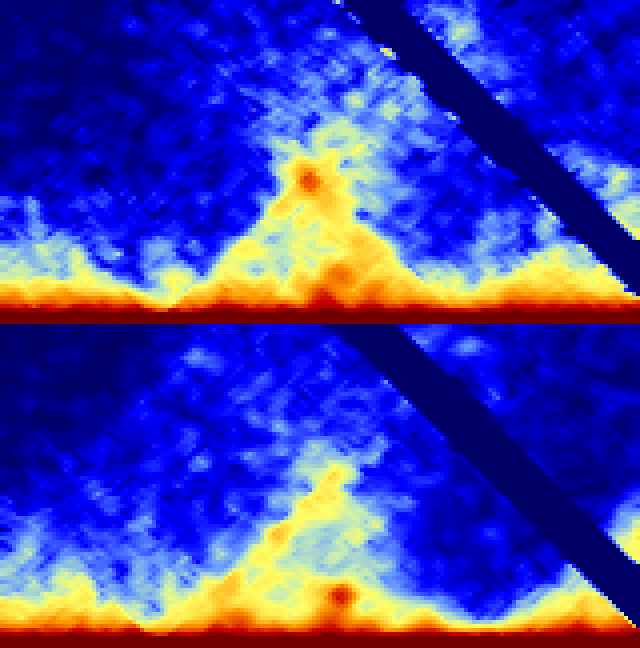
Visualizing Multiple Hi-C experiments
HOMER includes a script to help visualize matrices together to facilitate comparisons. The script batchMakeHiCMatrix.pl will take multiple Hi-C tag directories as input and report contacts in a single 'meta-matrix'. The script can be used to generate matrices in serial succession, split them along the diagonal, or to rotate them 45 degrees. In general, the command is run the following way:
batchMakeHiCMatrix.pl -pos <chr:start-end> -res <#> -window <#> [etc.] -d <HiCtagDir1> [HiCtagDir2] ...
#for example
batchMakeHiCMatrix.pl -pos chr21:42,550,000-42,950,000 -res 5000 -window 15000 -balance -cpu 2 -d MDM-HiC-Mock/ MDM-HiC-H5N1/ > outputMatrix.txt
The program will make matrices for all Hi-C tag directories using the same parameters for each experiment so that the results are comparable. Most of the parameters are passed directly to instances of analyzeHiC to generate the matrices. The program has 3 different ways to present the final matrices shown with examples below:
-stack (default) : simply concatenates the matrices on top of one another
batchMakeHiCMatrix.pl -pos chr21:42,550,000-42,950,000 -res 5000 -window 15000 -balance -cpu 2 -d MDM-HiC-Mock/ MDM-HiC-H5N1/ -stack > outputMatrix.txt
-split : Creates non-symmetric matrices where the lower left represents the first experiment and the upper-right represents the 2nd experiment. This methods is probably the sensitive (visually) for spotting differences between experiments. If additional experiments are provided, the 3rd and 4th will be split beneath the first two, and so on.
batchMakeHiCMatrix.pl -pos chr21:42,550,000-42,950,000 -res 5000 -window 15000 -balance -cpu 2 -d MDM-HiC-Mock/ MDM-HiC-H5N1/ -split > outputMatrix.txt
-rotate : Rotates matrices -45 degrees and places them in order on top of one another. This is approach works best when comparing 3 or more experiments. The one caveat with this approach is that it will only visualize a fraction of the original matrix such that the resulting rotated matrix does not get clipped at the corners. The additional option "-frac <#>" (default 0.33) controls if how much of the original matrix to consider (BTW, the dark blue strips in the example below are areas where there is a highly repetitive region):batchMakeHiCMatrix.pl -pos chr21:42,350,000-43,150,000 -res 5000 -window 15000 -balance -d MDM-HiC-Mock MDM-HiC-H5N1/ -cpu 30 -rotate -frac 0.5 > ~/ooo.txt
Command Line Options for analyzeHiC
Usage: analyzeHiC <PE tag directory> [options]...
Resolution Options:
-res <#> (Resolution of matrix in bp or use "-res site" [see below], default: 10000000)
-window <#> (size of region to count tags for overlapping windows, default: same as res)
Options for specifying the region to analyze:
-chr <name> (create matrix on this chromosome, default: whole genome)
-start <#> (start matrix at this position, default:0)
-end <#> (end matrix at this position, default: no limit)
-pos chrN:xxxxxx-yyyyyy (UCSC formatted position instead of -chr/-start/-end)
-chr2 <name>, -start2 <#>, -end2 <#>, or -pos2 (Use these positions on the
y-axis of the matrix. Otherwise the matrix will be sysmetric)
-p <peak file> (specify regions to make matrix, unbalanced, use -p2 <peak file>)
-vsGenome (normally makes a square matrix, this will force 2nd set of peaks to be the genome)
-chopify (divide up peaks into regions the size of the resolution, default: use peak midpoints)
-relative (use with -maxDist <#>, outputs diagonal of matrix up to maxDistance)
-pout <filename> (output peaks used for analysis as a peak file, -pout2 <file> for 2nd set)
Contact Matrix Options:
-ihskb <#> (normalize counts to "interactions per hundred square kilobases per billion, default)
Use -normTotal <#> and -normArea <#> to modify normalization constants, area in bp^2
-raw (report raw interaction counts)
-coverageNorm (Only adjust reads based on total interactions per region, default)
-balance (balance resulting matrix - row/column totals the same)
-distNorm (return log2 obs/expected counts normalized for interaction distance)
-corr (report Pearson's correlation coeff, use "-corrIters <#>" to recursively calculate)
-corrDepth <#> (merge regions in correlation so that minimum # expected tags per data point)
General options:
-o <filename> (Output file name, default: sent to stdout)
-compactionStats <output BEDGRAPH file prefix> (calculates DLR and ICF compaction scores)
-dlrDistance <#> (Cutoff distance for distal vs. local interactions for DLR, default: 3Mb
-ifc <outputFile> (outputs interaction frequence curve for regions, can set to "auto")
-4C <output BED file> (outputs tags interacting with specified regions)
-cpu <#> (number of CPUs to use, default: 1)
Filters & Other:
-nomatrix (skip matrix creation - use if more than 100,000 loci)
-std <#> (# of std deviations from mean interactions per region to exclude, default:8)
-min <#> (minimum fraction of average read depth to include in analysis, default: 0.05)
-minExpect <#> (minimum fraction of average read depth to use for coverage normalization, default: 0.75)
-override (Allow very large matrices to be created... be carful using this)
Older options:
Background Options:
-force (force the creation of a fresh genome-wide background model)
-bgonly (quit after creating the background model)
-createModel <custom bg model output file> (Create custome bg from regions specified, i.e. -p/-pos)
-model <custom bg model input file> (Use Custom background model, -modelBg for -ped)
-randomize <bgmodel> <# reads> (and the output is a PE tag file, initail PE tag directory not used
Use makeTagDirectory ... -t outputfile to create the new directory)
Older normalization options (often require creation of a background model):
-logp (output log p-values from old-style interaction calculations)
-expected (report expected interaction counts based on average profile)
-rawAndExpected <filename for expectd matrix> (raw counts sent to stdout)
-cluster (cluster regions, uses "-o" to name cdt/gtr files, default: out.cdt)
-clusterFixed (clusters adjacent regions, good for linear domains) Old interaction finding options (see findTADsAndLoops.pl):
-interactions <filename> (output interactions, add "-center" to adjust pos to avg of reads)
-pvalue <#> (p-value cutoff for interactions, default 0.001)
-zscore <#> (z-score cutoff for interactions, default 1.0)
-minDist <#> (Minimum interaction distance, default: resolution/2)
-maxDist <#> (Maximum interaction distance, default: -1=none)
-boundary <#> (score boundaries at the given scale i.e. 100000)
Comparing HiC experiments:
-ped <background PE tag directory>
Creating BED file to view with Wash U Epigenome Browser:
-washu (Both matrix and interaction outputs will be in WashH BED format)
Creating Circos Diagrams:
-circos <filename prefix> (creates circos files with the given prefix)
-d <tag directory 1> [tag directory 2] ... (will plot tag densities with circos)
-b <peak/BED file> (similar to visiualization of genes/-g, but no labels)
-g <gene location file> (shows gene locations)
Making Histograms:
-hist <#> (create a histogram matrix around peak positions, # is the resolution)
-size <#> (size of region in histogram, default = 100 * resolution)
Given Interaction Analysis Mode (no matrix is produced):
-i <interaction input file> (for analyzing specific sets of interactions)
-iraw <output BED filename> (output raw reads from interactions, or -irawtags <file>)
Command Line Options for batchMakeHiCMatrix.pl
batchMakeHiCMatrix.pl -pos <chr:start-end> -res
<#> -window <#> [etc.] -d <HiCtagDir1>
[HiCtagDir2] ...
Options:
-d <HiC TagDir1> [HiC TagDir2] ... (Tag Directories
of Hi-C experiments to visulize)
-pos <chr:start-end> (genomic position to visualize)
-res <#> (resolution of step size to use for
analysis)
-window <#> (resolution of window size for
aggregating interactions)
-balance (balance resulting Hi-C matrix)
-stack (Stacks matricies on top of one another i.e. square
and symetric, non-rotated, default)
-split (Creates split matricies i.e. square, non-symetric,
non-rotated)
(printed in order of directories: 1\2 3\4 5\6 ...)
-rotate (Rotates matrices, default)
-frac <#> (fraction of square matrix to consider for
rotating, default: 0.333)
-cpu (number of different processes to use, def: 1)
Other options are passed to analyzeHiC to control the
creation of the matrices

Can't figure something out? Questions, comments, concerns, or other feedback:
cbenner@ucsd.edu