HOMER

Software for motif discovery and next-gen sequencing analysis

MED263: GRO-Seq, START-seq, and Hi-C Exercises

This tutorial will walk you through an example of GRO-seq/START-seq analysis using HOMER and provide some pointers for using Juicebox to view Hi-C data.  This exercise builds off the previous exercise looking at ChIP-seq data in mouse ES cells (link to the previous exercise). Just as with the ChIP-seq exercise, it starts with aligned SAM files (only reads from mouse chr17) for a GRO-seq and START-seq experiment from ES cells and performs many of the basic analysis tasks that one might normally do when analyzing this type of data. This exercise does not really cover the gritty details of Hi-C processing and analysis - this is significantly more complicated to cover in a single class session.  However, it does introduce the use of Juicebox to view and interpret Hi-C data. More information about processing Hi-C data can be found in the HOMER documentation or Juicer Documentation (there are several other tools for processing Hi-C data too!).

In-class GRO-seq/START-seq & Hi-C tutorial:

0. Align FASTQ reads using bwa, bowtie2 or similar genome alignment algorithm.  This will produce a SAM or BAM file that can be analyzed using HOMER. The tutorial below also assumes HOMER is already installed and the mm9 genome is loaded.

1. Download the zip file containing SAM alignment files and unzip the archive.

wget -O samfiles.groseq.zip http://homer.ucsd.edu/homer/workshops/170209-MED263/samfiles.groseq.zip
unzip samfiles.groseq.zip

# If you don't have the files from the ChIP-seq exercise, download them too
wget -O samfiles.zip http://homer.ucsd.edu/homer/workshops/170209-MED263/samfiles.zip
unzip samfiles.zip

The archive should contain the following SAM files that have been aligned to the mouse mm9 genome:

# These are the files in the samfiles.groseq.zip file
groseq.chr17.sam
startseq.chr17.sam
ctcf.chr17.sam

# These are from the ChIP-seq exercise (i.e. samfiles.zip)
h3k27ac-esc.chr17.2m.sam
h3k4me2-esc.chr17.2m.sam
input-esc.chr17.2m.sam
klf4-esc.chr17.2m.sam
oct4-esc.chr17.2m.sam
sox2-esc.chr17.2m.sam

The GRO-seq and START-seq experiments are originally from the following study investigating the roles of proximal promoter pausing of RNA polymerase in the control of embryonic stem cell gene expression:

Pausing of RNA Polymerase II Regulates Mammalian Developmental Potential through Control of Signaling Networks
Sequencing Data: GSE43390

For this tutorial we analyze the GRO-seq and START-seq experiments (and ChIP-seq for the boundary/insulator protein CTCF) from mouse ESC (embryonic stem cells).  To reduce runtimes, only reads that mapped to chr17 are included in the SAM files.

2. As with ChIP-seq data, HOMER has several programs and routines to handle the analysis of GRO-seq and START-seq data.  The analysis of each data type starts the same way, with the creation of a "tag directory" that organizes the mapped sequencing information. Create a tag directory for the GRO-seq, START-seq and CTCF ChIP-seq experiment.  If you haven't already create tag directories for the data from the ChIP-seq exercise, create tag directories for those experiments too. The makeTagDirectory command has the following form:

makeTagDirectory <Output Tag Directory> [options] <input SAM file1> [input SAM file2] ...

You can see a full list of program options by simply running the command without any options. To create a tag directory for the GRO-seq experiment, run the following command with recommended options:

makeTagDirectory ESC-GROseq-mm9 -genome mm9 -checkGC groseq.chr17.sam

The command will take several seconds to run.  What it is doing is parsing through the SAM file, removing reads that do not align to a unique position in the genome, separating reads by chromosome and sorting them by position, calculating now often reads appear in the same position to estimate the clonality (i.e. PCR duplication), calculating the relative distribution of reads relative to one another to estimate the fragment length, calculating sequence properties and GC-content of the reads, and performs a simple enrichment calculation to check if the experiment looks like a ChIP-seq or an RNA-seq experiment.  In the case of GRO-seq (and strand specific RNA-seq in general), it is much harder for the program to estimate the fragment length without annotation.

The command creates a new directory, in this case named "ESC-GROseq-mm9".  Inside the directory are several text files that contain various QC results.  Try opening the following in a spreadsheet program (like open office or Excel):

tagInfo.txt - summary information from the experiment, including read totals
tagFreqUniq.txt - nucleotide frequencies relative to the 5' end of the sequencing reads.
gcContent.txt - distribution of ChIP-fragment GC%
tagAutocorrelation.txt - relative distribution of reads found on the same strand vs. different strands.
tagCountDistribution.txt - number of reads appearing at the same positions.

Repeat this command to create tag directories for the START-seq and CTCF ChIP-seq experiments:

makeTagDirectory ESC-STARTseq-mm9 -genome mm9 -checkGC startseq.chr17.sam
makeTagDirectory ESC-CTCF-mm9 -genome mm9 -checkGC ctcf.chr17.sam

#Also, if you haven't created them from the ChIP-seq exercise and homework:
makeTagDirectory ESC-Input-mm9 -genome mm9 -checkGC input-esc.chr17.2m.sam
makeTagDirectory ESC-Oct4-mm9 -genome mm9 -checkGC oct4-esc.chr17.2m.sam
makeTagDirectory ESC-Sox2-mm9 -genome mm9 -checkGC sox2-esc.chr17.2m.sam
makeTagDirectory ESC-Klf4-mm9 -genome mm9 -checkGC klf4-esc.chr17.2m.sam
makeTagDirectory ESC-H3K27ac-mm9 -genome mm9 -checkGC h3k27ac-esc.chr17.2m.sam
makeTagDirectory ESC-H3K4me2-mm9 -genome mm9 -checkGC h3k4me2-esc.chr17.2m.sam

Now try opening the "tagFreqUniq.txt" report files found in the CTCF, GRO-seq, and START-seq tag directories with a spreadsheet program (i.e. Excel) and graphing the nucleotide frequencies (i.e. first 5 columns).  These reveal the base composition relative to the 5' end of each read in the experiment.  Notice anything different about the different experiments.  Notice any unusually features in the START-seq output?

3. Next we will visualize the experiments by creating bedGraph files from the tag directories and using the UCSC genome browser to look at the results.  We will do this using the makeUCSCfile command.  This will work a little differently for each of the experiments do to the different nature of the experiments.  Both GRO-seq and START-seq provide strand specific information about the RNA that they are measuring, so we want to separate the reads that appear on each strand to consider them separately.  In addition, the START-seq reads specify the exact nucleotide where transcription initiation (i.e. the 5' end of the read).

First, create a bedGraph file from the CTCF ChIP-seq experiment in the same manner that we did for the ChIP-seq exercise:

makeUCSCfile ESC-CTCF-mm9 -o auto

This creates the file "ESC-CTCF-mm9/ESC-CTCF-mm9.ucsc.bedGraph.gz".  This file format specifies the normalized read depth at variable intervals along the genome (use zmore and the filename to view the file format for yourself). To view the file in the genome browser, do the following:

1. Visit https://genome.ucsc.edu/ with your internet browser.
2. In the top menu, click on "Genomes" -> "Mouse NCBI37/mm9" to go to the mouse mm9 version of the genome.
3. In the top menu, click on "My Data" -> "Custom Tracks".
4. In the "Paste URLs or data" input field, upload the ESC-CTCF-mm9.ucsc.bedGraph.gz file from the tag directory and hit submit.

Once the file finishes uploading, click go to go to the genome browser and start surfing the genome.  The read pileups will display the relative density of ChIP-seq reads at each position in the genome.  REMEMBER that we only have data for chr17 in this example, so stick to that chromosome.

Next we want to create visualization files for GRO-seq. HOMER's makeUCSCfile command contains an optional parameter called "-style rnaseq" that sets several options to streamline the creation of RNA-seq/GRO-seq visualization files.  Unlike the default, specifying "-style rnaseq" will split the reads up based on the strand they align to and set their fragment length for visualization to be equal to the length of the sequencing reads (this can also be used to visualize normal RNA-seq data):

makeUCSCfile ESC-GROseq-mm9/ -style rnaseq -o auto

This creates the file "ESC-GROseq-mm9/ESC-GROseq-mm9.ucsc.bedGraph.gz".  Load this file into the genome browser the same way you would load a ChIP-seq file.  In this case you'll notice that there are actually two new tracks added - one for the +strand reads and one for the -strand reads.  If you want to flip the -strand reads to be negative (i.e. extend down instead of up), right click on the track and select the "Negate Values" check box.

Now we will create visualization files for START-seq. Unlike for GRO-seq, we are mostly interested in the exact 5' end of the reads, so it can be useful to visualize the exact nucleotides that the reads start on instead of viewing the full coverage of the sequencing read. To accomplish this, use the "-style tss" option instead of "-style rnaseq".

makeUCSCfile ESC-STARTseq-mm9/ -style tss -o auto

As with the GRO-seq tracks, we can flip the -strand reads by right clicking on the track and selecting the "Negate Values" checkbox. You may want to drag the tracks up or down to order them next to one another (i.e. make sure the START-seq +strand and START-seq -strand are next to each other).

At this point it is worth it to cruise around chr17 and look at the data - notice how each of the different data types is distributed across the genome.  Can you see evidence for enhancer RNA?  What about promoter antisense RNAs?  What about signal in the GRO-seq data that extends past the 3' end of genes.  Try zooming into a promoter region to see the exact nucleotides where transcription starts based on the START-seq (For example, the Srsf3 promoter).  Hit the "base" next to the zoom in buttons at the top of the browser to zoom down to the nucleotide level to see the actual sequences near the initiation sites.  Can you find promoters that initiate transcription from a single, dominant initiation site and promoters that initiate from several different sites (i.e. sharp vs. broad initiation profiles).

4. Next, look at the distribution of sequencing reads relative to annotated transcription start sites to get a sense for if these experiments worked.  Similar to the ChIP-seq data from the last exercise, we'll use annotatePeaks.pl with the "tss" key word to create histograms.  The other modification we will make is the use of the option "-tbp <#>" which limits the tags per bp considered at each location when compiling the histogram.  This is important because GRO-seq and START-seq data are more quantitative than many other forms of NGS data such that we don't normally want to mark PCR duplicates during the analysis.  However, some promoters may have thousands of reads at a single bp, which will drown out the signal from other regions.  To help adjust for this, we can use "-tbp 1" or "-tbp 5" (for example) to limit the number of reads we consider at each position from a given region.  To generate a histogram around annotated TSS, run the following command:

annotatePeaks.pl tss mm9 -size 2000 -hist 10 -tbp 1 -d ESC-GROseq-mm9/ ESC-STARTseq-mm9/ > output.histogram.txt

Open the output.histogram.txt file in a spreadsheet program/Excel and create an X-Y line plot using the columns for the + tags and -tags from the START-seq and GRO-seq experiments.  Do you see evidence for upstream transcription from promoters?

5. As with ChIP-seq data, we can look for 'enriched' regions in the START-seq data to identify transcription start sites in data independent of previous annotations. We can use the same HOMER command called findPeaks to analyze the START-seq tag directories to identify TSS. The basic idea is that it looks for regions (300 bp in size) with high density of START-seq reads in a strand specific manner. It will also try to filter peaks with too much local background that can arise from non-capped small RNA fragments generated from the degradation products of highly expressed genes.  After findPeaks identifies TSS, it will recenter the peaks on the single initiation site with the highest signal. 

findPeaks ESC-STARTseq-mm9 -style tss -o auto

This command will generate a file called "tss.txt" in the ESC-STARTseq-mm9 folder.  This file contains the locations of each TSS discovered in the data.  HOMER also contains a routine for identifying transcription unites from GRO-seq data (i.e. "-style groseq"), but the example GRO-seq dataset used in this analysis has some biases in it that make analyzing it in this fashion not very useful (you can try it yourself though!). 

In addition to finding TSS from START-seq, we need to find peaks in our CTCF ChIP-seq data set too. Remember to use the "-style factor" to inform the program that we're analyzing transcription factor ChIP-seq data.

findPeaks ESC-CTCF-mm9 -i ESC-Input-mm9 -style factor -o auto

6. Next we will identify which TSS from our analysis of START-seq are located in putative enhancer elements.  To identify promoter-distal TSS elements, we can run a command called "getDistalPeaks.pl" to identify which peaks are found greater than 3kb from annotated promoters.  This command essentially runs the annotatePeaks.pl program to find the closest TSS and filters the peaks that are found too close.

getDistalPeaks.pl ESC-STARTseq-mm9/tss.txt mm9 > tss.enhancers.txt

Now the TSS found in enhancers will be stored in the "tss.enhancers.txt" file.  Approximately ~70% of the TSS should have come from enhancers.

7. Now lets look at the chromatin and TF landscape near enhancer initiation sites.  Do do this, lets create a histogram using the annotatePeaks.pl program again, but this time use the tss.enhancers.txt file as the input peaks/BED file:

annotatePeaks.pl tss.enhancers.txt mm9 -size 4000 -hist 10 -d ESC-Oct4-mm9/ ESC-Sox2-mm9/ ESC-Klf4-mm9/ ESC-H3K27ac-mm9/ ESC-H3K4me2/ ESC-CTCF-mm9/ > enhancer.histogram.txt

Open the "enhancer.histogram.txt" file with a spreadsheet program/Excel.  You'll notice that the first column gives the distance offsets from the TSS followed by columns corresponding to the 'coverage', '+ Tags', and '- Tags' for each experiment.  Try graphing each as X-Y line graph using the first column as the X-coordinate and graphing all of the "coverage" columns to see the patterns of each experiment. Where do the transcription factors appear relative to enhancer TSS?  How about this histone modification experiments?

8. To identify which regulatory motifs may be responsible for driving enhancer RNA expression, lets look for enriched motifs at our enhancer TSS locations.  This can be accomplished in a similar manner to how we look for motifs in ChIP-seq data with findMotifsGenome.pl.  However, given what is known about transcription factor binding relative to TSS (i.e. consider the graph from the previous step), we don't necessarily want to focus our search on the TSS but just upstream.  We can use the "-size" parameter to recenter where we search for motifs to be -150 to +50 relative to the TSS (the -S 10 and -len 10 parameters are included to speed up the execution by only looking for the top 10 motifs that are 10 bp long):

findMotifsGenome.pl tss.enhancers.txt mm9r Motifs-Enhancers/ -size -150,50 -p 10 -S 10 -len 10

Once the motif finding command finishes, do you notice anything interesting about the motifs identified? What is the top motif identified?

If you have time, consider running motif finding on the CTCF ChIP-seq dataset as well:

findMotifsGenome.pl ESC-CTCF-mm9/peaks.txt mm9r Motifs-CTCF/ -size 100 -p 10 -S 5

9. Now that you've found the most enriched motifs at enhancers, lets look at the distribution of the top motif (probably KLF4) relative to the enhancer TSS. As we did with the ChIP-seq results for Oct4, lets copy the top motif from the enhancer results to a easy location to use:

cp Motifs-Enhancers/homerResults/motif1.motif topMotif.motif

You should now have the file "topMotif.motif" in your current directory.  To see it's distribution relative to enhancer TSS, create another histogram to so that we can plot the distribution of the motif relative to the TSS:

annotatePeaks.pl tss.enhancers.txt mm9 -size 600 -hist 5 -m topMotif.motif > motif.histogram.enhancerTSS.txt

Open the "motif.histogram.enhancerTSS.txt" file with a spreadsheet program/Excel and plot the first two columns.  Where does the motif have a primary enrichment?  Now try plotting the motif relative to annotated TSS - is it similar?

annotatePeaks.pl tss mm9 -size 600 -hist 5 -m topMotif.motif > motif.histogram.geneTSS.txt

10. Now lets switch gears and start looking at Hi-C data. One of the best programs available at the moment to view Hi-C data is a program called JuiceBox, created by the Lieberman-Aiden laboratory. To run JuiceBox (can be run locally from your own computer if you want), download the application or Java JAR file from the following site:

http://aidenlab.org/juicebox/

During the class I will show you how to load data and auxiliary tracks, and how to compare data.

Homework:

This homework will build on the concepts from the ChIP-seq and GRO-seq/Hi-C classes to show how you can integrate findings across different types of data.  Below are questions found highlighted in RED - place the answers to the questions in a text file to turn in next week.

1. If you haven't already downloaded the files and followed the practical session above, download the files and work through the commands to produce the GRO-seq, START-seq, and CTCF tag directories, peak files, and UCSC visualization (bedGraph.gz) files.

2. Lets analyze the impact of CTCF and the directionality of its motif. To make the homework easier, lets standardize the CTCF motif (instead of doing de novo motif finding) and use HOMER's CTCF motif.  You can download the motif file from this link: ctcf.motif. Then run the following commands to identify the best possible motif match in each CTCF motif, returning a new peak file that is centered on the best CTCF motifs.

#first download the motif
wget -O ctcf.motif http://homer.ucsd.edu/homer/workshops/170209-MED263/ctcf.motif

#then find the best motif in each peak (NOTE: the -mscore option allows the motif to match suboptimal sites)
annotatePeaks.pl ESC-CTCF-mm9/peaks.txt mm9 -center ctcf.motif -mscore > ctcf.motifSites.txt

3. Now that we have identified the best CTCF motif matches in each peak, lets create a track for the genome browser that helps visualize each site and it's directionality.  The following script helps format the file from the last step and adds coloring so that it's easier to see which sites have a CTCF motif that orients to the + stand versus the - strand.

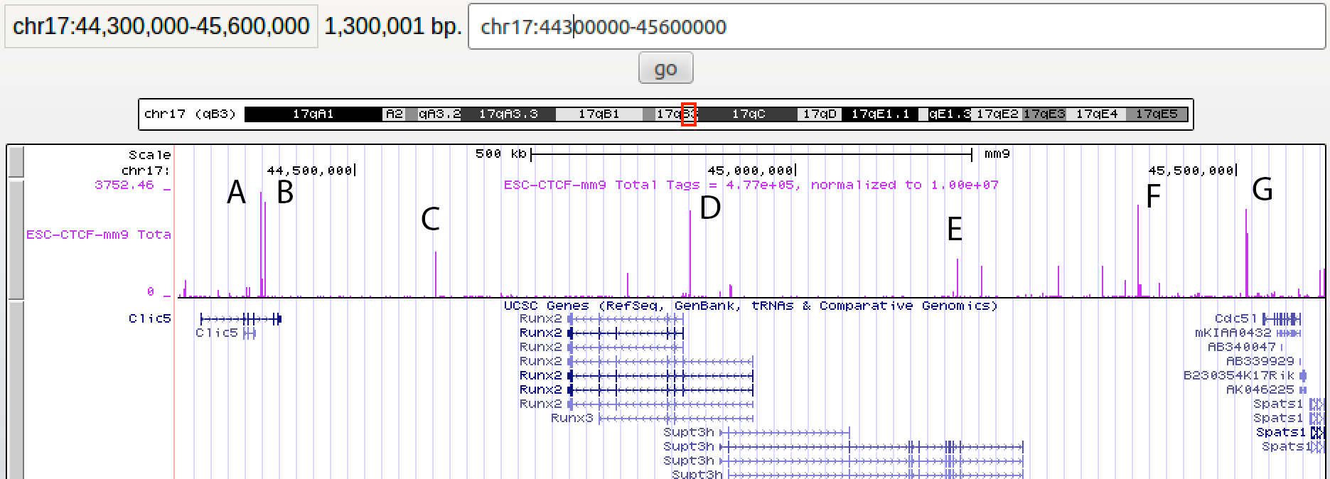
pos2bed.pl ctcf.motifSites.txt -track CTCF -color strand > ctcf.motifs.color.bed

4. Load the resulting BED file as a custom track into a UCSC Genome browser session.  Make sure you load the CTCF bedGraph we generated earlier, as well as the other tracks (hopefully they are already loaded from the class session). When looking at the CTCF motif positions, note that the RED sites are "- strand" and the BLUE are "+ strand" motifs.  Go to the following coordinates in the genome browser: chr17:44300000-45600000.  This is the Runx2/Supt3h locus, which is generally repressed in ES cells.

Q1: For each of the major CTCF peaks (i.e. tall peaks) found in this locus, record which ones are RED (i.e. -strand) and which ones are BLUE (i.e. +strand).  Give a value for each peak A,B,C,D,E,F, and G.

3. Next lets consider Hi-C data from the Juicebox application in the context of our other results.  Open Juicebox and load the Hi-C data files for mouse embryonic stem cells.  These are located in File->Open, and the file you want to look at is in the "Hi-C Data Archive (organized by year and first author) -> Dixon et al. | Nature 2012 -> mES -> HindIII combined (our alignment)".  This data will be presented in the same genome version and coordinate system used in our exercises.  Unfortunately, the data is not as dense and clean as the newer, deeply sequenced experiments we looked at in class.

4. Next load CTCF tracks to view alongside the ESC Hi-C data.  Go to "Annotations -> load ENCODE Tracks", and then find and select the "ES-Bruce4 ChIP-seq CTCF Signal bigWig LICR-m" row. This will cause the CTCF track to load at the top and left sides of the application.  You may want to right click on the track and change the settings to display the track as "max" instead of "average" and adjust the range to 0 to 30. Go to chr17 and zoom in on the the same region centered around 45 MB that were were looking at for CTCF peaks - the CTCF peaks in Juicebox should resemble the CTCF tracks you have in the UCSC genome browser for this region. You'll notice that this region contains a fairly large topological domain, with a smaller, dense domain in the middle.

Q2: Based on the Hi-C contact map in this region and the directionality of the major CTCF motifs, answer the following:
Do RED (i.e. -strand motifs) tend to make contact with chromatin upstream (i.e. to the left) or with chromatin downstream (i.e. to the right) relative to their genomic coordinates?
Do BLUE (i.e. +strand motifs) tend to make contact with chromatin upstream (i.e. to the left) or with chromatin downstream (i.e. to the right) relative to their genomic coordinates?

5. Now lets check if CTCF plays any type of role in transcription initiation.  More specifically, lets check to see if the direction of the CTCF plays a role in directing transcription initiation.  The CTCF motif positions we found in step 2 of this homework represent the CTCF motifs aligned on their 5' edges and oriented in the same direction.  To check if transcription is more likely to initiate on one side of the motif or the other, lets make a histogram relative to the CTCF motif sites:

annotatePeaks.pl ctcf.motifSites.txt mm9 -size 1000 -hist 1 -tbp 5 -di -d ESC-STARTseq-mm9/ > histogram.txt

You'll notice we're using a couple different values for some of the options.  First, we'll use "-hist 1" to generate a histogram at single bp resolution.  Second, we'll set "-tbp 5" to make sure super highly expressed TSS don't drown out the signal from other sites.  Third, we include the option "-di" to have it output nucleotide and dinucleotide frequencies so that we can verify the we are actually looking at the aligned CTCF motifs.

Open the output file with a spreadsheet program and create an X-Y line graph with column 1 (or A) as the x-axis and columns 3,4,5,6,7, and 8 (i.e. B-G) as the Y-coordinates.  Columns 3 and 4 show the transcriptional activity in the + and - strand relative to the motif, while Columns 5-8 show the nucleotide frequency.

Q3: Is the transcription initiation signal from START-seq higher upstream (i.e. - strand) or downstream (i.e. + strand) relative to the CTCF motif.  At what distance from the 5' edge of the motif is the signal the strongest?

Q4: CTCF often binds to sites that have a very long motif that extends past the core ~20bp sequence that we used to predict binding sites. Looking at the nucleotide frequencies of the sequences around the core DNA motif (i.e. 0-19 bp), are the sequence preferences stronger in the region from -40 to -20 or are they they stronger from +20 to +40?

Q5: Given your answer to Q2 and Q3 above, and knowing that the data in this file are all sites oriented relative to the +strand of CTCF motifs (i.e. 0 is the 5' of CTCF motifs oriented in the + strand), does transcription near CTCF normally initiate toward the center of TADs, or 'away' from TADs? In other words, does transcription initiate at CTCF sites in the same direction that they tend to form loops in, or in the opposite direction?