HOMER

Software for motif discovery and next-gen sequencing analysis

Chromatin Compartment Analysis (PCA)

Quick Reference for PCA analysis

#PCA of Hi-C contact matrices essentially clusters apart the 'checkerboard' pattern to reveal active and inactive chromatin regions along the genome:
runHiCpca.pl auto HicExp1TagDir/ -res 25000 -window 50000 -genome hg38 -cpu 10

#This will create two files in the tag directory, *.PC1.bedGraph and *.PC1.txt.  The *.PC1.bedGraph file can be viewed in a Genome Browser. If you have ChIP-seq or other regions that you know represent 'active regions', replace "-genome hg38" with something like "-active K27ac.peaks.bed"
#If your sequencing depth is low, you may need to use "-res 50000 -window 100000"

#To compare multiple experiments, first run runHiCpca.pl on each tag directory. Once you have several PCA analysis from multiple experiments, you can combine their quantification into a single spreadsheet:
annotatePeaks.pl HiCExp1TagDir/HiCExp1TagDir.PC1.txt hg38 -noblanks -bedGraph HiCExp1TagDir/HiCExp1TagDir.PC1.bedGraph HiCExp2TagDir/HiCExp2TagDir.PC1.bedGraph HiCExp3TagDir/HiCExp3TagDir.PC1.bedGraph > output.txt

#If you have PC1 bedGraphs from replicate experiments across two conditions, you can identify significantly changing compartments using the following:
annotatePeaks.pl Exp1r1.PC1.txt hg38 -noblanks -bedGraph Exp1r1.PC1.txt Exp1r2.PC1.txt Exp2r1.PC1.txt Exp2r2.PC1.txt > output.txt
getDiffExpression.pl output.txt exp1 exp1 exp2 exp2 -pc1 -export outputPrefix > output2.txt

#In the example above, "exp1 exp1 exp2 exp2" labels the groups/replicates in the order that they appear in the input file

Principal Component Analysis of Hi-C Data

PCA is a powerful technique for analyzing high dimensional data, and first used on Hi-C data by Lieberman-Aiden et al.  The basic idea behind PCA is to redefine the coordinate system such that the data can be "described" with as few dimensions as possible (a type of clustering or dimensionality reduction).  The new axes of the coordinate system are referred to as the principle components, and the "1st" component is found such that it can be used to describe or discriminate as much of the variance in the data as possible, with the "2nd" component describing as much of the remaining variance as possible, and so on.  We can then consider each region with respect to their values along the first couple principal components to get a simplified view of the data.

To perform PCA on Hi-C data, we apply it to the distance-normalized interaction matrix. In this setting, each region along the chromosome represents a dimension in the analysis.  Normally, PCA is applied to full chromosome matrices to identify important features.  You could apply PCA to the entire genome interaction matrix, but sparse interactions between chromosomes may introduce too much noise.  You can also apply PCA to a small region, although the conclusions from such an analysis are less general with respect to general chromosome structure and what we normally think of as chromatin compartments.

To perform PCA analysis with HOMER, use the program runHiCpca.pl.  Below is an example:

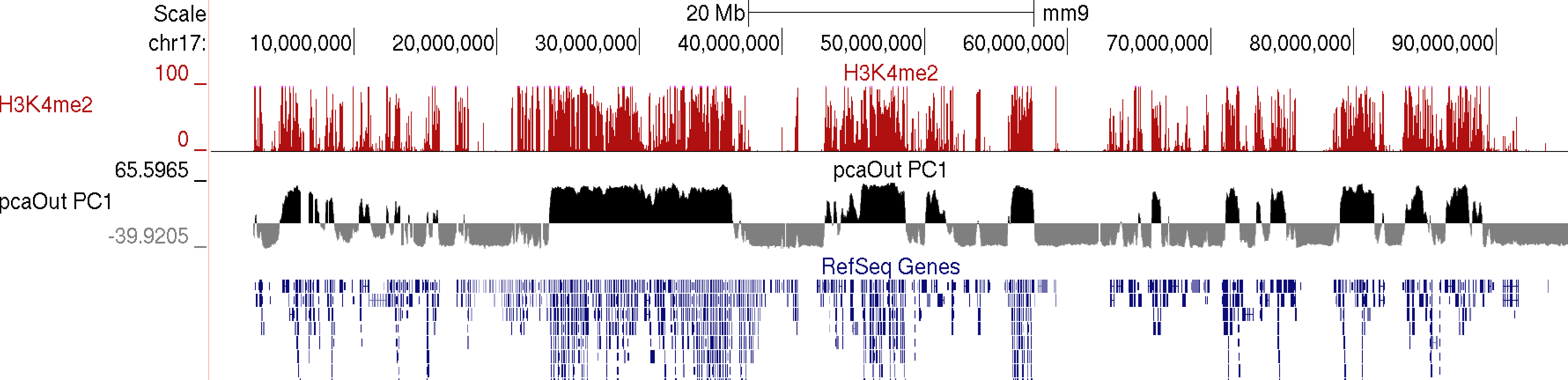
runHiCpca.pl <outputPrefix> <HiC Tag Directory> [options]

example: runHiCpca.pl pcaOut ES-HiC/ -res 50000 -cpu 4 -genome mm9

This command will produce two output files: *.PC1.txt and *.PC1.bedGraph (i.e. pcaOut.PC1.bedGraph). If the first argument is "auto", the files will be named the same as the tag directory and placed directly in the tag directory (useful when analyzing experiment in batch). The bedGraph file can be directly uploaded to UCSC or similar genome browser and represents the coordinates of each region with respect to the first principle component (PC1).  The txt file contains the same information in peak file format.  Below is an example of the output on chr17:



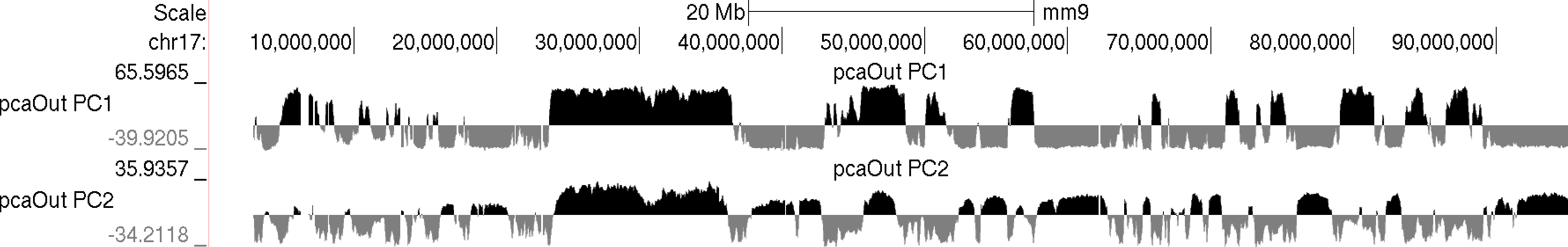
Usually the values for the first principal component (PC1) are the most informative.  These indicate the classification of each region of the chromosome with respect to the first component.  Normally, gene-rich regions with 'active' chromatin marks have similar PC1 values, while gene deserts tend to have similar but opposite loadings from the active regions.  You can also view additional principal components by changing the "-pc <#>" option to a higher number.  The 2nd component (PC2) usually describes the the location along the chromosome (e.g. near telomere vs. centromere, or different chromosome arms).  The PC2 values tend look a lot like the PC1 values but usually "flip" along the length of the chromosome.  Their similarity is partly due to the fact that they are mathematically linked - Each principal component must be orthogonal to one another, so unless the first PC1 perfectly describes a feature of the data, other PCs might reflect the feature as well.  In the example below, PC1 and PC2 values are more similar for the first 40 Mb, and then they tend to be more opposite for the rest of the chromosome.




In general, this analysis tends to highlight the fact that the genome can be divided into two compartments, creating a "checkerboard" pattern, with positive PC1 regions reflecting "active/permissive" chromatin and negative PC1 regions indicative of "inactive/inert" chromatin

What does runHiCpca.pl do:

runHiCpca.pl is a wrapper script that will perform PCA analysis on each chromosome individually and combine all the results.  Below are each of the steps:

1. Check for the appropriate background model for distance normalized contact normalization, create it if necessary.

2. For each chromosome:

- Generate distance normalized (-distNorm) interaction matrix (analyzeHiC)
- Calculate correlation between the contact profiles from each region against each other region
- Using R, compute the principal components from the correlation matrix
- Output the values of reach region with respect to the first principal components

3. If "seed" regions are provided, HOMER checks the overlap between active (and/or inactive) regions to decide if the PC1 values should be multiplied by -1 to flip the signs.  HOMER will try to make it so regions in "active" zones are positive.  If no seed regions are used, but a genome is specified, HOMER will look for overlap with gene TSS locations to assign the active regions.

4. Concatenate results from all chromosomes, format, and print the output

runHiCpca.pl Options:

-pc <#> : Number of principal components to return (default: 1).

-res <#> : resolution of analysis (if it's too small, the program may take too long or use up too much memory).  A resolution of 25000 is about the limit for mammalian genomes, unless your computer is ridiculous... The sequencing depth and quality of an experiment may dictate which resolutions are possible.  If the PC1 values are very noisy you may need to increase the resolution size. Default: 50000

-window <#> : window size of analysis, should be equal to or larger than -res. Default: 100000.

-active <peak/BED file> : seed regions of "active" chromatin to use when assessing the proper sign of the PC1 results.

-inactive <peak/BED file> : seed regions of "inactive" chromatin to use when assessing the proper sign of the PC1 results.

-genome <genome> : If no seed regions are given, HOMER will get the TSS locations and treat them as "active" seeds.

-corrDepth <#> : Minimum number of expected reads per region to use when computing correlation (pools adjacent regions), default: 3

-std <#> : exclude regions with sequencing depth exceeding # std deviations, default: 4.  The idea here is to remove regions that may throw off the PCA calculation

-min <#> : exclude regions with sequencing depth less than this fraction of mean, default: 0.15.  The idea is to get rid of regions with low coverage that don't behave as well during the PCA analysis.

-rpath <path to R executable> : If "R" is not available through the $PATH variable (i.e. can't just type "R" to run R)

-cpu <#> : number of CPUs to use.  Memory consumption is also higher with more CPUs (work separated by chromosome).  Please note that if multiple CPUs are configured, the screen output will spew all over the place - just ignore it...

Advanced Options:

-customRegions <peak/BED file> : This option allows a user to specify which regions should be used for PCA analysis. By default, HOMER will analyze whole chromosomes, but in some cases this can be problematic. For example, in some cases chromosome arms on either side of the centromere have odd interaction patterns (perhaps due to the % of cells in mitosis), and sometimes genome duplications in cell lines introduces artifacts that are difficult to deal with in the analysis. An example of using this option would be to specify the coordinates for each chromosome arm separately as peaks:

chr1p   chr1    1       121535434       +
chr1q   chr1    124535434       249250621       +
chr10p  chr10   1       39254935        +
chr10q  chr10   42254935        135534747       +
...

Notes for PCA analysis with HOMER

Choosing the correct resolution/window parameters for PCA analysis can depend on the depth of sequencing. The smaller the resolution the noisier the analysis tends to get. The correct way to evaluate the proper resolution would be to sample half the data and repeat the analysis such that you get roughly the same results. The following rough guidelines can help though:

Sequencing Depth: res (window)
<200 million reads: 50000 (100000)
200 million -1 billion reads: 25000 (50000)
>1 billion: 10000 (20000)*
(in reality, PCA analysis eventually looses it's sensitivity - probably best to approach compartments using an alternative approach for higher resolutions)

Sometimes the PC1 values do not correspond to the active/inactive compartments that we normally expect to see in Hi-C data.  In some cases (i.e. mitotic chromatin) this may be expected.  In other cases, it's possible that genome duplications/translocations or inadequate sequencing depth result unexpected results. In these cases it's recommended to either try to increase the resolution/window sizes or to try to analyze the data by chromosome arm (i.e. -customRegions <peak/BED file> described above).

Another potential problem with PCA analysis is that sometimes the sign of the PC1 values is not correct (i.e. flipped). HOMER includes a script called "flipPC1toMatch.pl" which takes your PC1.bedGraph output and a 2nd PC1.bedGraph experiment that you want to match to, and will flip PC1 values by chromosome in the first file to match the 2nd file.

Comparing PC1 values across Experiments

Since chromatin compartments are often highly associated with transcription activity, it is usually a good idea to compare PCA results between different Hi-C experiments to check for evidence that compartment may change across samples. HOMER offers a relatively rigorous approach to differential PC1 analysis, and some more empirical solutions depending on the availability of replicates.

Creating a matrix of PC1 values to compare across experiments

After running "runHiCpca.pl" on all of your Hi-C experiments, it can be useful to have a single file containing the PC1 values for each region across each experiment. To do this, run annotatePeaks.pl with the "-bedGraph <file1> [file2]..." option using one of the PC1.txt files as the input peak/BED file (essentially provides peaks tiling the genome).  It is also recommended to add the option "-noblanks" to only include regions with PC1 value assignments across all experiments (i.e. no missing data) - this usually only removes a handful of regions near centromeres or other repetitive regions:

annotatePeaks.pl exp1.PC1.txt hg38 -noblanks -bedGraph exp1.PC1.bedGraph exp2.PC1.bedGraph exp3.PC1.bedGraph > output.txt

The resulting file can then be opened with Excel or similar program to look through the data.

Identifying statistically significant changes in chromatin compartments

If you have two or more replicates across different conditions, you can use HOMER's getDiffExpression.pl script to automate a differential analysis of PC1 values. Perform the following steps:

1. Perform the PCA analysis for all experiments separately

runHiCpca.pl auto HicExp1r1TagDir/ -res 25000 -window 50000 -genome hg38 -cpu 10
runHiCpca.pl auto HicExp1r2TagDir/ -res 25000 -window 50000 -genome hg38 -cpu 10
runHiCpca.pl auto HicExp2r1TagDir/ -res 25000 -window 50000 -genome hg38 -cpu 10
runHiCpca.pl auto HicExp2r2TagDir/ -res 25000 -window 50000 -genome hg38 -cpu 10

2. Create a single spreadsheet containing the PC1 values across all 4 experiments

annotatePeaks.pl HiCExp1TagDir/HiCExp1r1TagDir.PC1.txt hg38 -noblanks -bedGraph HiCExp1r1TagDir/HiCExp1r1TagDir.PC1.bedGraph HiCExp1r2TagDir/HiCExp1r2TagDir.PC1.bedGraph HiCExp2r1TagDir/HiCExp2r1TagDir.PC1.bedGraph HiCExp2r2TagDir/HiCExp2r2TagDir.PC1.bedGraph > output.txt

3. Run getDiffExpression.pl on the output from annotatePeaks.pl. With this command, the first argument is the input file, followed by experiment names that are used to annotated which columns in the file are replicate conditions. These should be entered in the same order that the bedGraph files were provided in the annotatePeaks.pl command.

getDiffExpression.pl output.txt exp1 exp1 exp2 exp2 -pc1 -export regions > diffOutput.txt

This command will run the values through limma to identify statistically significantly changing PC1 regions. You must specify "-pc1" in the command to trigger the PC1 analysis. This command will provide 3 output files. The first is the spreadsheet that is sent to stdout, which reports the difference in PC1, p-values, and adj. p-values for the changes in PC1 between experimental conditions for each region in the genome.  The 2nd and 3rd files start with the prefix "regions" in this case, and represent contiguous regions that are statistically different between conditions. These are found by stitching together individual regions exceeding the significance thresholds to yield regions of interest. The options parameters control how they are found:

PC1 Hi-C analysis options for stitching differentially scoring regions with getDiffExpression.pl:

-fdr <#> : (FDR/adj. p-value cutoff to use to identify significant regions, default: 0.05)
-log2fold <#> : (the difference in PC1 values to use to identify significant regions, default: 1, note that this is for the difference, not the log2 ratio)
-minRegionSize <#> : (minimum size of stitched region to report, def: 100000)
-bridgeDistance <#> : (maximum distance to merge sig. regions, def: 50000)
-minPosPC1 <#> : (Minimum value for A compartment PC1 values, def: 0)
-maxNegPC1 <#> : (Maximum value for B compartment PC1 values, def: 0)

Finding PC1 Based Compartments

Regions of continuous positive or negative PC1 values set the stage for identifying "compartments", in this case referring to linear regions of DNA that are in the "active/permissive" or "inactive/inert" compartments.  (This is a little different than the concept of topological domains reported in Dixon et al., which are more of a local phenomenon instead of a compartment association).

Note: Unlike the annotatePeaks.pl command, findHiCCompartments.pl works on the *.PC1.txt files that are produced by runHiCpca.pl, not the *.PC1.bedGraph files.

To identify compartments, run the command:

findHiCCompartments.pl exp1.PC1.txt > compartments.txt

By default, this command will identify all regions that have a continuous positive PC1 value.  The output is a peak file that contains each of these regions, their average PC1 value across the region, and their length in the 6th and 7th columns, respectively.  To adjust the threshold used to call compartments, use the "-thresh <#>" option.  To identify regions with negative PC1 values, add the "-opp" option to the command.  Also, if you prefer to return compartments as the original sub-peaks (instead of stitching them together into a single, long peak), add the "-peaks" option.

Differential Compartments without replicates

The findHiCCompartments.pl command also has some built in support for identifying regions that change their compartment between experiments.  Two sources of information can be used to identify changes: the PC1 values from a second Hi-C experiment, and/or the correlation difference (i.e. getHiCcorrDiff.pl output) between two experiments.  If both options are used, the identified regions must pass both criterion.

-bg <PC1.txt file> : specify a background experiment's PC1 results.
-diff <#> : minimum difference between PC1 values to define region as different, default: 50

-corr <corrDiff.txt file> : specify a correlation difference file
-corrDiff <#> : maximum correlation for a region to be defined as different, default: 0.4

Below is an example of these files uploaded to the UCSC Genome Browser. NOTE: If UCSC complains that you chromsome coordinates exceed the end of the chromosome (could happen due to the resolution), run the command "removeOutOfBoundsReads.pl compartments.txt <genome> > compartments.new.txt" to adjust the coordinates at the end of the chromosome.

Downstream PC1 analysis

There are several ways to use HOMER to analyze PC1 values (or corrDiff values) with respect to other data.  Some are very general ways to manipulate bedGraphs, while others are very specialized to PC1 values (i.e. getDomains.pl).

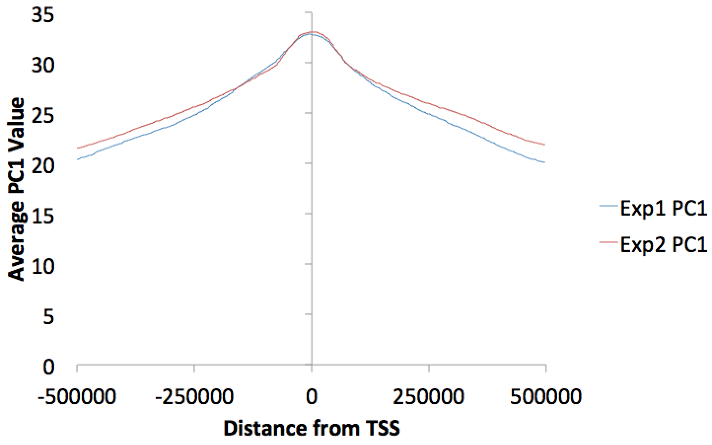
Histograms/Quantifying PC1 values at genomic features

You can make histograms of PC1 values around areas of interest by using annotatePeaks.pl and the "-bedGraph" option.  Lets say you'd like to see the distribution of PC1 values around TSS. (alternatively you could look at PC1 values near ChIP-Seq peaks or other features)  Using the command below:

annotatePeaks.pl tss mm9 -size 1000000 -hist 1000 -bedGraph exp1.PC1.bedGraph exp2.PC1.bedGraph > output.histogram.txt

Opening the histogram output in Excel and graphing the "coverage" columns:

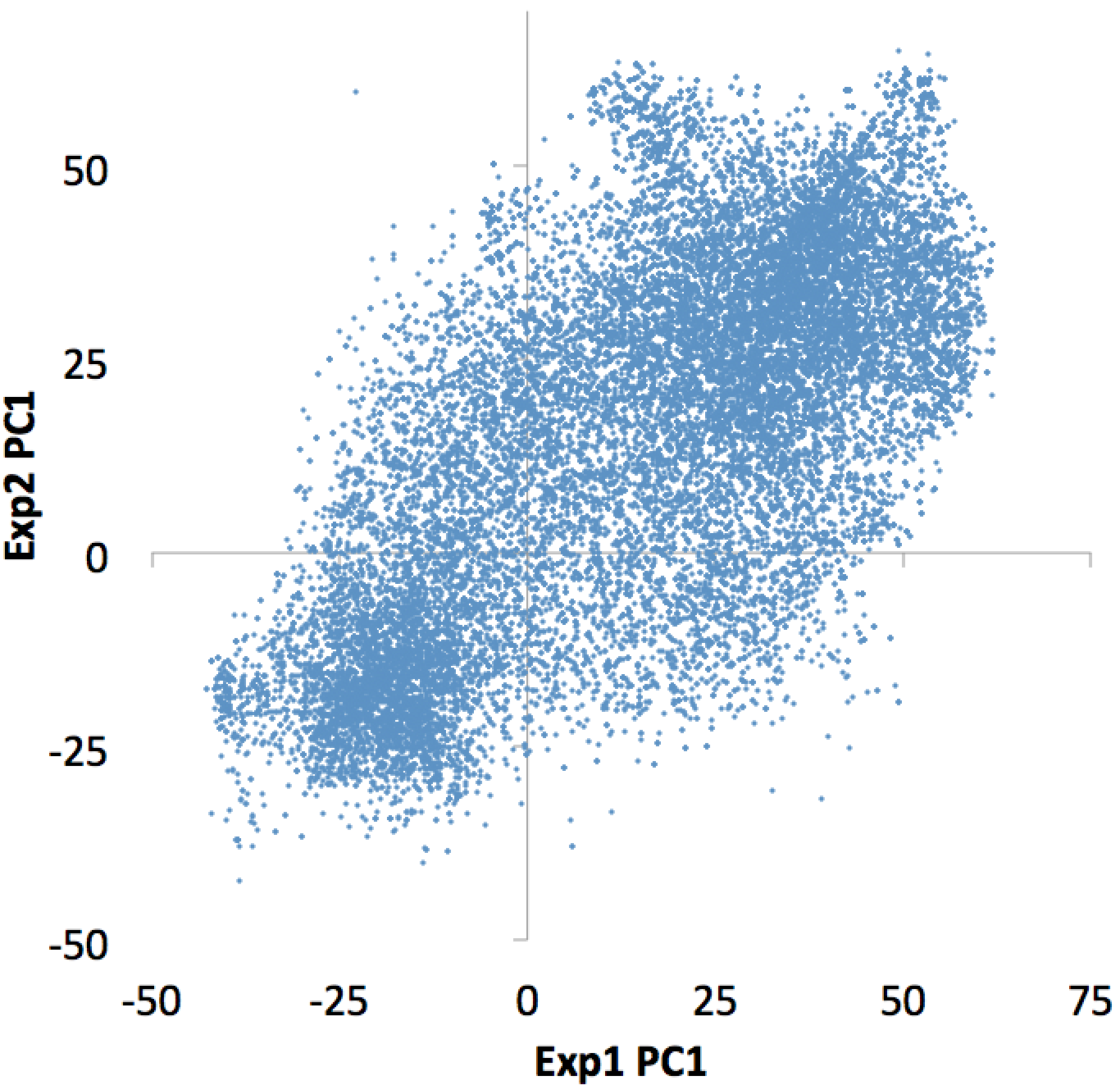
You can also omit the "-hist <#>" option and adjust the size from the annotatePeaks.pl command, and annotatePeaks.pl will instead quantify the PC1 values at each locus, which can be useful for classifying which TSS are in the 'active/permissive' compartment vs. which TSS are in the 'inactive/inert' compartment:

annotatePeaks.pl tss mm9 -size 1000 -bedGraph exp1.PC1.bedGraph exp2.PC1.bedGraph > output.table.txt

Opening this file with Excel:

Plotting the bedGraph data columns as a scatter plot:

This file can also be used to figure out which individual TSS are changing the most, etc.  Similar operations could be performed on ChIP-Seq peaks or other features of interest.

Directly Comparing Two Hi-C Experiments

PCA analysis is a useful tool for analyzing single Hi-C experiments.  However, comparing PC1 values between two experiments *can* be a little dangerous.  PCA is an unbiased method for data analysis, and while PC1 values usually correlated with "active" vs. "inactive" compartments, the precise qualitative nature of this association may differ slightly between experiments.  Because of this, HOMER offers another approach to directly compare the interaction profiles between two experiments rather than simply looking at PC1 values.

One way to do this is to directly correlate the interaction profile of a locus in one experiment to the interaction profile of that same locus in another experiment.  If the locus tends to interact with similar regions in both Hi-C experiments, the correlation will be high.  If the locus interacts with different regions in the two experiments, the correlation will be low.  Note that this is NOT PCA analysis, cut a direct comparison between two experiments at each locus.  By default, this will compare the interaction profiles across each chromosomes (interchromosomal interactions are generally too sparse for this type of analysis)

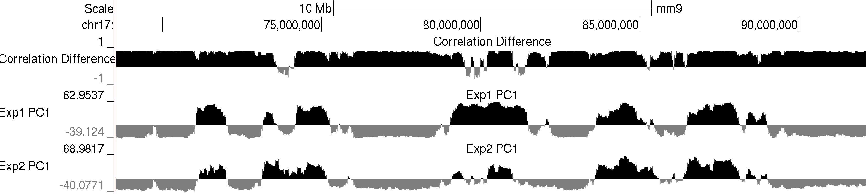
To calculate the "correlation difference" between two experiments, use the getHiCcorrDiff.pl.  Below is how it's used:

getHiCcorrDiff.pl <outputPrefix> <HiC Tag Directory1> <HiC Tag Directory2> [options]

example: getHiCcorrDiff.pl out ES-HiC Bcell-HiC -cpu 8 -res 50000

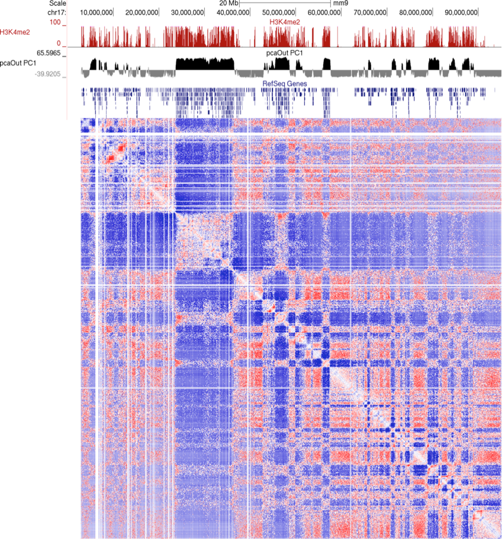
This program will produce two output files, much like runHiCpca.pl.  One is a bedGraph what can be loaded into the UCSC Genome Browser as a custom track.  The other is a peak file with the correlation information in the 6th column.  Below is an example of the corrDiff output loaded with the PC1 values from two experiments:

Additional Options for getHiCcorrDiff.pl:

-res <#> : resolution of analysis (if it's too small, the program may take too long or use up too much memory).  A resolution of 25000 is about the limit for mammalian genomes, unless your computer is ridiculous... The sequencing depth and quality of an experiment may dictate which resolutions are possible.  If the values are very noisy you may need to increase the resolution size. Default: 50000.

-superRes <#> : window size of analysis, should be equal to or larger than -res. Default: 100000.
               
-corrDepth <#> : Minimum number of expected reads per region to use when computing correlation (pools adjacent regions), default: 3

-std <#> : exclude regions with sequencing depth exceeding # std deviations, default: 4.  The idea here is to remove regions that may throw off the PCA calculation

-min <#> : exclude regions with sequencing depth less than this fraction of mean, default: 0.15.  The idea is to get rid of regions with low coverage that don't behave as well during the PCA analysis.

-maxDist <#> : By default, getHiCcorrDiff.pl compares each locus by looking at it's contact profile across the whole chromosome.  Setting this option will limit the profile comparison to the region +/- this distance from the locus (sort of like a 'local' correlation)

-cpu <#> : number of CPUs to use.  Memory consumption is also higher with more CPUs (work separated by chromosome).  Please note that if multiple CPUs are configured, the screen output will spew all over the place - just ignore it...

Command Line Options for runHiCpca.pl

Command Line Options for getHiCcorrDiff.pl

Command Line Options for findHiCCompartments.pl